It is well known that sound waves travel through different gases at different speeds. Perhaps the most popular demonstration of this phenomenon are the modulated voices of people who have inhaled Helium ¹.

The goal of this post is to understand how the molecular composition of a gas determines the speed of sound waves passing through it. To make sure we are grounded in reality, we would specifically like to explain this table of the speed of sound through various gases from the Handbook of Chemistry and Physics ². These speeds are for gases at standard atmospheric pressure (1 atm) and the indicated reference temperatures.

Name	Formula	Molar Mass (g/mol)	Temperature (C)	Speed (m/s)
Carbon Dioxide	$CO_2$	44.01	0	258
Ammonia	$NH_3$	17.031	0	414
Neon	$Ne$	20.179	0	433
Helium	$He$	4	0	973
Ethane	$C_2H_6$	30.07	27	312
Argon	$Ar$	39.948	27	323
Oxygen	$O_2$	31.999	27	330
Dry Air		28.96	25	346
Nitrogen	$N_2$	28.01	27	353
Methane	$CH_4$	16.04	27	450
Hydrogen	$H_2$	2.01	27	1320

After staring at this table a bit a few trends emerge. First of all, the speed of sound seems to decrease as the mass of the gas increases. But clearly mass is not the only relevant factor. For example, Argon is heavier than Ethane but sound travels more quickly through Argon. The same is true for Neon and Ammonia.

How can we make sense of these outliers? Note that in both cases the lighter molecule nevertheless contains more atoms. For example, a molecule of Ethane has 8 atoms whereas the noble Argon has only one. So perhaps the number of atoms is what determines the speed of sound, where a greater number of atoms implies a lower speed?

This second hypothesis fails as well. For example, Methane has more atoms than Argon but the speed of sound through Methane is greater.

To make sense of these data, we will develop a simple model describing sound waves and use it to derive a formula for the speed of sound using Newton’s laws of motion and basic thermodynamics. We’ll then test our model on the table above and find that it is surprisingly accurate!

Based on the experimental success of our model we’ll conclude that the speed of sound in an ideal gas depends on three factors: temperature, mass and heat capacity. As we will explain later in more detail, heat capacity is essentially a proxy for the number of atoms. The general idea is that molecules can absorb energy into the vibrations and rotations of their constituent atoms relative to one another. So molecules with more atoms have more opportunities to absorb heat.

In the next section we study what happens when a wave passes through a series of balls connected by springs. The key result will be a formula for the speed of such a wave in terms of the mass of the balls and the stiffness of the springs.

We will then show that a pneumatic tube filled with gas behaves quite similarly to a spring. Using the ideal gas law and the first law of thermodynamics we’ll see that the “stiffness” of such a spring is determined by the temperature and heat capacity of the gas.

Finally, we’ll put everything together to write down a formula for the speed of sound in a gas in terms of its mass, temperature and heat capacity and verify that it is consistent with the table.

The Ball and Spring Model

Sounds waves are an example of a compression wave. In this section we will study a simpler model of compression waves and extend our results to sound waves later.

Our model consists of a series of balls connected by springs as in the diagram below:

The balls all have the same mass which we denote by $m$. Similarly, all of the springs have the same stiffness $k$ and length $h$.

What happens if we squeeze the springs on one of the ends? Here is a simulation comparing two systems of 100 balls. The only difference between the systems is that the springs in the top one have stiffness $k=1$ whereas the bottom ones have stiffness $k=10$. Each line represents a ball and the springs have been omitted for clarity. Also, a few of the “balls” have been colored red to make it easier to track their motion but they are physically identical to the rest of the balls.

The simulation starts with the ten leftmost springs compressed. These springs push back, compressing the springs to their right. Then those springs push back against their neighbors and eventually the springs on the right side become compressed. We call this propagation of compression a compression wave.

Note that when the wave in the bottom model with $k=10$ reaches the other side (i.e, when the right end is compressed), the top model with $k=1$ has only gone about $1/3$ of the way. In other words, the wave in the $k=10$ model travels about $3$ times as fast.

The goal for the remainder of this section will be to derive a formula for the speed of a compression wave in the ball and spring model in terms of the mass $m$, spring stiffness $k$ and spring length $h$. If the formula is any good then hopefully it will predict the speed difference we observed in the simulation.

Let’s start by analyzing how far each ball deviates from equilibrium at time $t$. In our model, the equilibrium position for ball $i$ is $x = i \cdot h$. We define $u(x, t)$ to be equal to the amount that the ball with equilibrium position $x$ has moved by time $t$. For example, $u(4\cdot h, 10)$ records the amount that ball $4$ has moved from its equilibrium at time $t=10$.

To make things more concrete, here is a graph of $u(x, t)$ for the $k=10$ model in the previous simulation. To make the numbers nicer to look at, in this simulation we are measuring $x$ in terms of multiples of $h$ and $t$ is the frame index.

As you can see, at $t=0$, $u(10, 0) = -9$ which corresponds to the fact that the $10$th ball has been pulled to the left by $9h$ meters. The balls nearby have also been shifted to a lesser degree. But $u(x, 0) = 0$ for $x \geq 20$ which means that all the balls to the right of ball $20$ start in their equilibrium position. After $30$ frames things are different. Now $u(10, 30)$ is close to zero whereas $u(90, 30)$ is around $8$ indicating that now the rightmost springs are compressed.

If the relationship between the springs below and the graph above is not clear, it may be helpful to focus on one of the lines highlighted in red and observe how the dot above it on the graph moves up and down as the line vibrates right and left.

To understand how compression waves propagate we will analyze how $u(x, t)$ evolves over time. Let’s start by focusing on the ball with equilibrium position $x$:

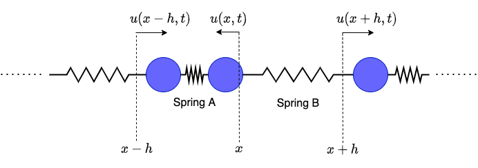
How much force is exerted on the middle ball of the diagram at time $t$? First lets consider “Spring A”. The right end of the spring has been displaced by $u(x, t)$ and the left end has been displaced by $u(x-h, t)$. Together this means that spring A has been stretched by $u(x, t) - u(x-h, t)$. Therefore by Hooke’s Law the force exerted by spring A on the ball is: \[ F_A = -k \cdot (u(x, t) - u(x-h, t))
\]

Similarly, the force exerted by “Spring B” is: \[ F_B = k \cdot (u(x + h, t) - u(x, t))
\]

There is no minus sign in this case because the force is to the right. Therefore, the total force on the ball is: \[ F = F_A + F_B = k \cdot (u(x + h, t) - 2u(x, t) + u(x - h, t)) \]

Multiplying and dividing by $h^2$ we get: \[ F = k h^2 \cdot \frac{(u(x + h, t) - 2u(x, t) + u(x - h, t))}{h^2} \]

But as $h\rightarrow 0$, the fraction on the right converges to the second derivative of $u(x, t)$ with respect to $x$ so: \begin{equation}\label{eq:force} F = kh^2 \frac{\partial^2 u}{\partial x^2} \end{equation}

By Newton’s second law, the force on the ball is related to the acceleration $\frac{\partial^2 u}{\partial t^2}$ by: \begin{equation}\label{eq:accel} F = m \cdot \frac{\partial^2 u}{\partial t^2} \end{equation}

Finally, let’s define a constant $c$ by: \[ c = \sqrt{\frac{kh^2}{m}} \]

Combining equations \ref{eq:force} and \ref{eq:accel} we get the famous wave equation: \[ \frac{\partial^2 u}{\partial t^2} = c^2 \frac{\partial^2 u}{\partial x^2} \]

We’ll now show that the speed of the wave is actually equal to $c$! To see why this is so, let’s try to find some functions $u(x, t)$ that satisfy the wave equation. As a warm up, here is one possible solution: \[ u(x, t) = \cos(x - c\cdot t) \]

To verify that this is a valid solution, we calculate some derivatives

and find that indeed \[ \frac{\partial^2}{\partial t^2}\cos(x - c\cdot t) = c^2 \frac{\partial^2}{\partial x^2}\cos(x - c\cdot t) \]

With a bit more analysis one can show that all solutions to the wave equation are of the form: \[ u(x, t) = f(x + ct) + g(x - ct) \]

where $f$ and $g$ are arbitrary single variable functions. But notice that $g(x - ct)$ represents the function $g(x)$ shifting to the right with speed $c$ and $f(x + ct)$ is the function $f(x)$ shifting to the left with speed $c$. In conclusion, all solutions $u(x, t)$ to the wave equation propagate with speed $c$, even the complicated looking one in our simulation above.

To summarize, we have found that compression waves propagate through the ball and spring model with a speed of: \begin{equation}\label{eq:c} c = \sqrt{\frac{kh^2}{m}} \end{equation}

How well does this match our simulations at the beginning of the section? Recall that we observed that the wave in the model with $k=10$ travelled around three times faster than the wave in the $k=1$ model. On the other hand our formula predicts that if $m$ and $h$ are fixed, the speed of the wave is proportional to $\sqrt{k}$. That implies that the ratio of the speeds in our simulation should be $\frac{\sqrt{10}}{\sqrt{1}}$ which is indeed close to three!

Making a Spring out of Gas

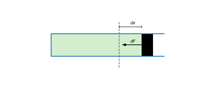
We now relate the ball and spring model to sound by replacing the springs with tubes of gas. Consider a tube which is filled with gas and sealed at the end by a piston. As part of this model we will also assume that the the tube is thermally insulated from the environment.

In the equilibrium state, the pressure in the tube is equal to the atmospheric pressure so the piston is stationary. But when the piston is displaced it oscillates around the equilibrium point as though it were connected to a spring:

The reason for this is that when the piston is pulled out the pressure in the tube decreases and so the piston is pushed back in. Similarly, if the piston is pressed in the pressure inside increases and the piston is pushed back out. In the simulation above, a darker color indicates a higher pressure.

The goal of this section is to formalize this analogy by computing the stiffness $k$ of a pneumatic tube in terms of properties of the gas inside.

By definition, stiffness measures the degree to which the piston resists small deformations. To be concrete, suppose we slightly displace the piston by $dx$ meters. Then the force pushing the piston back will be equal to

\begin{equation}\label{eq:piston-hooke} dF = -k \cdot dx \end{equation}

So to compute $k$ we must determine how the change in force $dF$ depends on the change in position $dx$.

Let $A$ denote the area of the piston, $p_a$ denote the atmospheric pressure and $p$ the pressure in the tube. Then the force on the piston is equal to $F = A \cdot (p - p_a)$. Therefore: \begin{equation}\label{eq:piston-dF} dF = A \cdot dp \end{equation}

Furthermore, let $V$ denote the volume of the tube and let $V_0$ denote the volume at equilibrium. Then $V = V_0 + A\cdot dx$ which means that: \begin{equation}\label{eq:piston-dx} dx = \frac{dV}{A} \end{equation}

Putting together equations \ref{eq:piston-hooke}, \ref{eq:piston-dF} and \ref{eq:piston-dx} we find that $A \cdot dp = -k \cdot \frac{dV}{A}$ or in other words: \begin{equation}\label{eq:piston-k} k = -A^2 \frac{dp}{dV} \end{equation}

Thus, to compute the stiffness $k$ me must compute the derivative of the pressure with respect to volume at the equilibrium. Before we continue, note that $-\frac{dp}{dV}$ is indeed a very reasonable measure of stiffness. If $-\frac{dp}{dV}$ is big then decreasing the volume of the tube by $dV$ will cause a large increase in pressure inside the tube meaning that then pressing on the tube will be very difficult.

Recall that the interior of the tube is thermally insulated from the environment. This type of process is called adiabatic. A fundamental result in thermodynamics states that an ideal gas going through an adiabatic process satisfies the following equation ³: \begin{equation}\label{eq:adiabatic} pV^{\gamma} = \mathrm{constant} \end{equation}

where $\gamma$ is the adiabatic index of the gas. This result follows fairly easily from the first law of thermodynamics as you can see in the reference. We will discuss the adiabatic index in more detail later, but for now we’ll simply note that it is roughly inversely proportional to the gas’s heat capacity.

Differentiating equation \ref{eq:adiabatic} with respect to $V$ around the equilibrium values of $V = V_0$ and $p = p_0$ gives us: \[ V_0^\gamma \frac{dp}{dV} + p_0\gamma V_0^{\gamma - 1} = 0 \]

which means that \begin{equation}\label{eq:dpdV} \frac{dp}{dV} = -\gamma\frac{p_0}{V_0} \end{equation}

Plugging this into equation \ref{eq:piston-k} gives us our formula for the stiffness of a pneumatic tube: \begin{equation}\label{eq:piston-k-final} k = \gamma A^2 \frac{p_0}{V_0} \end{equation}

Calculating the Speed of Sound

We will now merge the ball and spring model with the pneumatic tubes to compute the speed of sound in a gas. Specifically, we will compute the speed of a sound wave propagating through a long cylinder of gas with cross section $A$.

Sound waves are examples of compression waves. For instance, suppose someone claps their hand on the left side of the cylinder. This will displace the gas at that end and cause it to become compressed. This compressed gas will push back and end up compressing the gas next to it and so on. Here is a simulation in which a darker color indicates a more compressed gas:

To relate this to the ball and springs model, lets subdivide the cylinder into many smaller tubes each with the same number of molecules:

Observe the similarity to our ball and spring simulations! Specifically, we can think of the walls as “balls” which are separated by springs created out of gas as in the previous section. As a crude approximation, we will assume that the mass $m$ in each tube is concentrated on its left wall.

What is the stiffness coefficient of these springs? Let $p_0$ denote the equilibrium pressure of the gas, $h$ the equilibrium length of the tubes and $V_0$ their equilibrium volume. By equation \ref{eq:piston-k-final} the stiffness is:

\[ k = \gamma A^2 \frac{p_0}{V_0} \]

By equation \ref{eq:c} this means that the speed of compression waves propagating through the gas is: \[ c = \sqrt{\gamma A^2 \frac{p_0}{m V_0} h^2} \]

Using the relationship $V_0 = hA$ we can simplify this to: \begin{equation}\label{eq:sound-c} c = \sqrt{\gamma \frac{p_0 V_0}{m} } \end{equation}

where as before, $m$ is the mass of the gas in each tube.

According to the ideal gas law ⁴: \[ pV = nRT \]

where $n$ is the number of molecules in a tube (in moles), $R = 8.314\, \mathrm{JK}^{-1}\mathrm{mol}^{-1}$ is the ideal gas constant and $T$ is the temperature in Kelvin. Plugging this into equation \ref{eq:sound-c} leaves us with:

\begin{equation}\label{eq:sound-c-2} c = \sqrt{\gamma \frac{nRT}{m} } \end{equation}

Finally, let $M$ be the mass of one mole of gas molecules measured in kilograms (aka the molar mass). By definition this means that $M$ is equal to the mass of a tube divided by the number of molecules in the tube in moles: $M = \frac{m}{n}$. We can therefore simplify equation \ref{eq:sound-c-2} to:

\begin{equation}\label{eq:sound-c-3} c = \sqrt{\gamma \frac{RT}{M} } \end{equation}

Now that we have a precise formula for the speed of sound, we can test it on the table of speeds that we puzzled over in the introduction! Here is another version of the table where we have added a column for the adiabatic index which we looked up in HCP ² and a column containing the speed of sound as predicted by equation \ref{eq:sound-c-3}.

Name	M (kg/mol)	$\gamma$	T (K)	Speed (m/s)	$\sqrt{\gamma \frac{RT}{M} }$
Carbon Dioxide	0.044	1.289	273.15	258	257
Ammonia	0.017	1.310	273.15	414	418
Neon	0.020	1.666	273.15	433	434
Helium	0.004	1.666	273.15	973	972
Ethane	0.030	1.188	300.15	312	314
Argon	0.039	1.666	300.15	323	326
Oxygen	0.031	1.394	300.15	330	335
Nitrogen	0.028	1.400	300.15	353	353
Methane	0.016	1.304	300.15	450	450
Hydrogen	0.002	1.406	300.15	1320	1324

The agreement between the experimentally observed speeds and our formula is quite remarkable! This reinforces our theory that the speed of sound in an ideal gas depends only on the temperature, mass and the adiabatic index.

It makes sense that a wave would have a harder time traveling through a gas with heavier molecules. But what does the adiabatic index have to do with it? In the next section we will discuss the index in more detail and develop some intuition for why a higher adiabatic index implies a faster speed of sound.

Heat Capacity and the Adiabatic Index

In the previous section we showed that the speed of sound in a gas is proportional to its adiabatic index. The technical reason for this is equation \ref{eq:piston-k-final} which says that the adiabatic index determines the gas’s stiffness. But what is the adiabatic index and what does it have to do with stiffness?

In this section we interpret the adiabatic index in terms of the more intuitive concept of heat capacity and then try to understand the connection between heat capacity and the compressibility of a gas.

For starters, the adiabatic index of an ideal gas can be expressed in terms of the gas’s heat capacity ⁵: \begin{equation}\label{eq:gamma-cv} \gamma = 1 + \frac{R}{c_V} \end{equation}

As before, $R$ is the ideal gas constant. The interesting term here is $c_V$ which denotes the heat capacity of one mole of gas at a constant volume - also known by the fancier name of the isochoric specific heat.

Intuitively, the heat capacity of a gas measures the amount of energy that each molecule can store internally. Common types of internal energy are vibrations and rotations of the molecule’s atoms with respect to one another. Heat capacity has units of Joules per Kelvin and kilogram: $J/(K\, kg)$. I.e, the amount of energy that can be stored in a kilogram of the material for each degree Kelvin.

As an example, let’s compare Helium ($He$) to Ethane ($C_2H_6$).

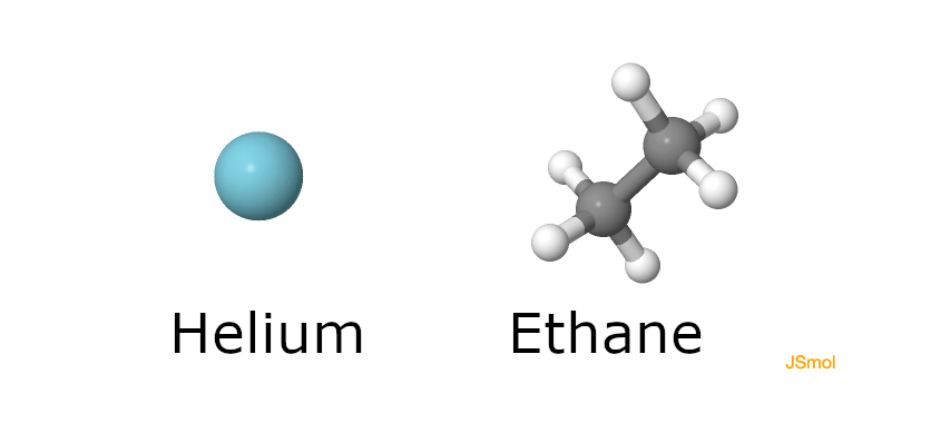
Ethane molecules each have 8 atoms and clearly there are many interesting ways for them to rotate and vibrate relative to one another. In contrast, Helium molecules are quite lonely with only a single atom. And indeed, the specific heat of Ethane is $44.186\, J/(K\, kg)$ whereas the specific heat of Helium is only $12.486 J/(K\, kg)$.

What does this have to do with stiffness?

We claim that a tube filled with Helium is harder to compress, i.e stiffer, than a tube of Ethane with the same volume. To see why, first imagine pressing down on the Helium tube. This pressing is a form of work which increases the energy of the Helium molecules. Since Helium molecules have a relatively low heat capacity, most of this energy will be used to increase the molecule’s kinetic energy rather than their internal energy.

Now let’s imagine pressing on the Ethane tube. As before, this will increase the energy of the Ethane molecules. But in this case, a lot of the energy will used to increase the internal energy of the molecules - for example by spinning them around or vibrating bonded pairs of atoms. Therefore comparatively little energy will be left over for the kinetic energy.

The end result is that the Helium molecules will be moving faster than the Ethane molecules. As a consequence the pressure in the Helium tube will be greater thus making it harder to compress.

Coming back to the speed of sound, recall that in our analysis of the ball and spring model we found that the speed of a compression wave is proportional to the stiffness of the springs. Since gases with lower heat capacity like Helium are “stiffer”, sound waves travel through them more quickly.

In summary, we’ve seen that the speed of sound in a gas depends on its temperature, mass and heat capacity. If the gas molecules have a larger mass then they are harder to move which makes sound travel more slowly. If the gas has a lower heat capacity then it reacts more forcefully to compression which causes sound to propagate more quickly. We formalized this relationship in equation \ref{eq:sound-c-3} and found that it agrees quite nicely with experimental evidence!

---