Fully Homomorphic Encryption from Scratch
03 Jan 2024
Introduction
Fully Homomorphic Encryption (FHE) is a form of encryption that makes it possible to evaluate functions on encrypted inputs without access to the decryption key. For example, suppose you want to use a neural network running on an untrusted server to determine whether your image contains a cat. Since the server is untrusted, you do not want it to see your image. With FHE you can encrypt the image with your secret key and upload the encrypted image to the server. The server can then apply its neural network to the encrypted image and produce an encrypted bit. You can then download the encrypted bit and decrypt it with your secret key to obtain the result.
In other words, FHE makes it possible to leverage the computational resources of an untrusted server without having to send it any unencrypted data.
At first glance it seems like FHE is impossible. Encrypted data should be indistinguishable from random bytes to a person without access to the encryption key. So how could such a person perform a meaningful calculation on the encrypted data?
In this post we will explore a popular FHE encryption scheme called TFHE and implement it from scratch in Python. All of the code in this post together with tests can be found here: https://github.com/lowdanie/tfhe
The standard cryptography exposition disclaimer applies. Namely, that it probably is not a good idea to copy paste code from this post to secure your sensitive data. You can use the official TFHE library instead.
A Fully Homomorphic NAND Gate
Any boolean function can be implemented with a combination of NAND gates. Therefore, in this post we’ll focus on implementing a homomorphic version of the NAND gate which can be evaluated on encrypted inputs.
Specifically, we’ll implement generate_key, encrypt and decrypt functions:
def generate_key() -> EncryptionKey:
    pass

def encrypt(plaintext: Plaintext, key: EncryptionKey) -> Ciphertext:
    pass

def decrypt(ciphertext: Ciphertext, key: EncryptionKey) -> Plaintext:
    pass
and a homomorphic NAND gate:
def homomorphic_nand(
    ciphertext_left: Ciphertext,
    ciphertext_right: Ciphertext,
) -> Ciphertext:
    """Homomorphically evaluate the NAND function."""
    pass
The homomorphic property will allow us to perform the following type of computation:
# Client side: Create an encryption key and encrypt two bits.
client_key = generate_key()

b_0 = True
b_1 = False

ciphertext_0 = encrypt(b_0, client_key)
ciphertext_1 = encrypt(b_1, client_key)

# The client sends the ciphertexts to the server.

# Server side: Compute an encryption of NAND(b_0, b_1) from
# the two ciphertexts:
ciphertext_nand = homomorphic_nand(ciphertext_0, ciphertext_1)

# The server sends ciphertext_nand back to the client.

# Client side: Decrypt ciphertext_nand.
# The result should be equal to NAND(True, False) = True
result = decrypt(ciphertext_nand, client_key)
assert result
Importantly, the server never receives the client_key and so it is not able to
read the contents of ciphertext_left or ciphertext_right. Nevertheless, it
can run the homomorphic_nand function on the ciphertexts to produce
ciphertext_nand which encrypts NAND(b_0, b_1). Without the client_key, the
server cannot read the contents of ciphertext_nand. All it can do is send
ciphertext_nand back to the client who can use their client_key to decrypt
it and reveal the result.
Of course, all of this complexity is unnecessary if the client is only interested in evaluating a single NAND gate. The client would be better off just evaluating the NAND function locally not involving a server at all.
Homomorphic encryption becomes more useful when the client wants to evaluate a
complex circuit such as a neural network which is composed of many billions of
NAND gates. In that case the client may not have the compute or the permission
to run the program locally. Instead they can offload the computation to an
untrusted server using the approach in the code snippet above, where the
homomorphic_nand function is used by the server to evaluate each of the NAND
gates in the complex circuit.
The goal of this post is to implement generate_key, encrypt, decrypt and
homomorphic_nand.
Learning With Errors
In this section we wil implement generate_key, encrypt and decrypt. This
combination of functions is typically called an Encryption Scheme.
Encryption schemes are usually based on a fundamental mathematical problem that is assumed to be “hard”. For example, RSA is based on the assumption that is is hard to find the prime factors of large integers. Similarly, TFHE is based on a problem called Learning With Errors (LWE). In the next section we will define the LWE problem and use it to construct an encryption scheme.
As we will see, in the LWE encryption scheme it is possible to homomorphically add ciphertexts but not to homomorphically multiply them. This type of encryption scheme is called Partially Homomorphic because not all operations are supported. Despite this limitation, the partially homomorphic operations in the LWE scheme will be useful stepping stones on the path towards fully homomorphic encryption.
In this section we will define the Learning With Errors (LWE) problem and use it to implement our encryption scheme as well as some homomorphic operations.
Notation
Let $q$ be a positive integer. We will denote the integers modulo $q$ by $\mathbb{Z}_q := \mathbb{Z} / q\mathbb{Z}$. In this post, it will be convenient to set $q=2^{32}$ so that elements of $\mathbb{Z}_q$ can be represented by the signed 32-bit integers: $[-2^{31}, 2^{31})$. One advantage of using 32-bit integers is that all operations are natively done modulo $2^{32}$.
Similarly, $\mathbb{Z}_8$ will denote the integers modulo $8$. We will identify $\mathbb{Z}_8$ with the set of integers $[-4, 4)$.
The Learning With Errors Problem
Let $\mathbf{s} \in \mathbb{Z}^n_q$ be a length $n$ vector with elements in $\mathbb{Z}_q$ which is assumed to be secret. Let $\mathbf{a}_1, \ldots , \mathbf{a}_m \in \mathbb{Z}^n_q$ be random vectors and let $b_i = \mathbf{a}_i \cdot \mathbf{s}$ be the dot product of $\mathbf{a}_i$ with $\mathbf{s}$. As a warmup to the LWE problem we can ask:
Given $m \geq n$ random vectors $\mathbf{a}_1,\dots,\mathbf{a}_m$ and the dot products $b_i, \ldots , b_m$, is it possible to efficiently learn the secret vector $\mathbf{s}$?
It is not hard to see that the answer is “yes”. Indeed, we can create an $m \times n$ matrix $A$ whose rows are the vectors $\mathbf{a}_i$ and a length $m$ vector $\mathbf{b}$ whose elements are $b_i$:
\[ A = \begin{bmatrix} \mathbf{a}^T_1 \\ \vdots \\ \mathbf{a}^T_m \end{bmatrix}_{m \times n} \mathbf{b} = \begin{bmatrix} b_1 \\ \vdots \\ b_m \end{bmatrix} \]
We can then express $\mathbf{s}$ as the solution to the linear equation:
\[ A \mathbf{s} = \mathbf{b} \]
Finally, we can use Gaussian Elimination to solve for $\mathbf{s}$ in polynomial time. Note that the standard Gaussian elimination algorithm has to be tweaked a bit to account for the fact that $\mathbb{Z}_q$ is not a field - but the general idea is the same.
We can think of the above problem as Learning Without Errors since we are given the exact dot products $b_i = \mathbf{a}_i \cdot \mathbf{s}$. It turns out that if we introduce errors by adding a bit of noise $e_i$ to each $b_i$, then learning $\mathbf{s}$ from the random vectors $\mathbf{a}_i$ and the noisy dot products $b_i = \mathbf{a}_i \cdot \mathbf{s} + e_i$ is very hard. We can now state the Learning With Errors problem:
Given $m$ random vectors $\mathbf{a}_1, \ldots , \mathbf{a}_m$ and noisy dot products $b_i = \mathbf{a}_i \cdot \mathbf{s} + e_i$, is it possible to efficiently learn the secret vector $\mathbf{s}$?
Note that we have not yet specified which distribution the errors $e_i \in \mathbb{Z}_q$ are drawn from. In TFHE, they are sampled by first sampling a real number $-\frac{1}{2} \leq x_i < \frac{1}{2}$ from a Gaussian distribution $\mathcal{N}(0, \sigma)$ with $\sigma \ll 1$, and then scaling $x$ by $q$ to obtain a number in the interval $[-\frac{q}{2}, \frac{q}{2})$ and finally rounding to the nearest integer:
\[\begin{equation}\label{eq:int-noise} e = \lfloor x \cdot \frac{q}{2} \rfloor \end{equation}\]We will denote the distribution on $\mathbb{Z}_q$ obtained in this way by $\mathcal{N}_q(0, \sigma)$.
In the next section we will see how to build a partially homomorphic encryption scheme based on the hardness of LWE.
An LWE Based Encryption Scheme
Following the notation of the previous section, our encryption scheme will be parameterized by a modulus $q$, a dimension $n$ and a noise level $\sigma$. Typical values would be $q=2^{32}$, $n=500$ and $\sigma=2^{-20}$.
The valid inputs to an encryption function are known as the message space. The message space of the LWE scheme is $\mathbb{Z}_q$. We will also call valid messages plaintexts.
The encryption keys are random length $n$ binary vectors $\mathbf{s} \in \{0, 1\}^n \subset \mathbb{Z}^n_q$.
To encrypt a message $m \in \mathbb{Z}_q$ with a key $\mathbf{s} \in \mathbb{Z}^n_q$ we first uniformly sample a vector $\mathbf{a} \in \mathbb{Z}^n_q$ and sample a noise element $e\in\mathbb{Z}_q$ from the Gaussian distribution $\mathcal{N}_q(0, \sigma)$. The encrypted message, also known as the ciphertext, is defined to be the pair
\[ \mathrm{Enc}_{\mathbf{s}}(m) := (\mathbf{a}, \mathbf{a} \cdot \mathbf{s} + m + e) \in \mathbb{Z}_q^n \times \mathbb{Z}_q \]
If we know the secret key $\mathbf{s}$, we can decrypt a ciphertext $(\mathbf{a}, b)$ by computing:
\[ \mathrm{Dec}_{\mathbf{s}}((\mathbf{a}, b)) = b - \mathbf{a} \cdot \mathbf{s} = (\mathbf{a} \cdot \mathbf{s} + m + e) - \mathbf{a} \cdot \mathbf{s} = m + e \]
In section Message Encoding we’ll describe a method for removing the error term $e$ in the equation above so that we can recover the exact message $m$ after decryption.
Note that the encryption function is not deterministic since it samples from the distribution $\mathcal{N}_q(0, \sigma)$. It turns out that this is a feature and not a bug. Indeed, any semantically secure encryption scheme must have a non-deterministic encryption function. To see why, suppose we use the scheme to encrypt yes/no responses to a poll. If the encryption function was deterministic, we could tell if two people voted the same way by comparing their encrypted responses. In a non-deterministic scheme, this attack no longer works since even two people that voted the same way will have different encrypted responses.
Let $m$ be an LWE plaintext. Since the encryption function is non-deterministic, rather than saying that a ciphertext $L = (\mathbf{a}, b)$ is the encryption of $m$ we will say that it is an encryption of $m$. The set of valid encryptions of $m$ with key $\mathbf{s}$ will be denoted $\mathrm{LWE}_{\mathbf{s}}(m)$. If $L = \mathrm{Enc}_{\mathbf{s}}(m)$ then $L$ is an encryption of $m$ and so we can write:
\[ L \in \mathrm{LWE}_{\mathbf{s}}(m) \]
Here is an implementation of the LWE encryption scheme:
import dataclasses

import numpy as np

from tfhe import utils
@dataclasses.dataclass
class LweConfig:
    # Size of the LWE encryption key.
    dimension: int

    # Standard deviation of the encryption noise.
    noise_std: float


@dataclasses.dataclass
class LwePlaintext:
    message: np.int32


@dataclasses.dataclass
class LweCiphertext:
    config: LweConfig
    a: np.ndarray  # An int32 array of size config.dimension
    b: np.int32


@dataclasses.dataclass
class LweEncryptionKey:
    config: LweConfig
    key: np.ndarray  # An int32 array of size config.dimension


def generate_lwe_key(config: LweConfig) -> LweEncryptionKey:
    return LweEncryptionKey(
        config=config,
        key=np.random.randint(
            low=0, high=2, size=(config.dimension,), dtype=np.int32
        ),
    )


def lwe_encrypt(
    plaintext: LwePlaintext, key: LweEncryptionKey
) -> LweCiphertext:
    a = utils.uniform_sample_int32(size=key.config.dimension)
    noise = utils.gaussian_sample_int32(std=key.config.noise_std, size=None)

    # b = (a, key) + message + noise
    b = np.add(np.dot(a, key.key), plaintext.message, dtype=np.int32)
    b = np.add(b, noise, dtype=np.int32)

    return LweCiphertext(config=key.config, a=a, b=b)


def lwe_decrypt(
    ciphertext: LweCiphertext, key: LweEncryptionKey
) -> LwePlaintext:
    return LwePlaintext(
        np.subtract(ciphertext.b, np.dot(ciphertext.a, key.key), dtype=np.int32)
    )
where the utils module contains:
from typing import Optional

import numpy as np

INT32_MIN = np.iinfo(np.int32).min
INT32_MAX = np.iinfo(np.int32).max


def uniform_sample_int32(size: int) -> np.ndarray:
    return np.random.randint(
        low=INT32_MIN,
        high=INT32_MAX + 1,
        size=size,
        dtype=np.int32,
    )


def gaussian_sample_int32(std: float, size: Optional[float]) -> np.ndarray:
    return np.int32(INT32_MAX * np.random.normal(loc=0.0, scale=std, size=size))
Throughout this post, we will used the following LweConfig whose parameters
are taken from the popular
Lattice Estimator.
from tfhe import lwe

LWE_CONFIG = lwe.LweConfig(dimension=1024, noise_std=2 ** (-24))
Ciphertext Noise
Let $m \in \mathbb{Z}_q$ be an LWE plaintext and let $\mathbf{s}$ be an LWE encryption key. Let $L \in \mathrm{LWE}_{\mathbf{s}}(m)$ be an LWE encryption of $m$. In the previous section we saw that:
\[ \mathrm{Dec}_{\mathbf{s}}(L) = m + e \]
where $e$ is some small noise whose magnitude depends on the LWE parameters. In other words, when we decrypt $L$ we get the original message $m$ together with a small error term. We will call $e$ the noise in the ciphertext $L$.
As an example, we’ll use the code above to encrypt the message $m = 2^{29}$ one thousand times and plot a histogram of the ciphertext noise. We’ll use the LWE config above where the encryption noise has a standard deviation of $\sigma=2^{-24}$. Since we multiply this by $q/2 = 2^{31}$ during encryption following equation \ref{eq:int-noise}, we expect the ciphertext noise to have a standard deviation of roughly $\sigma’=2^{31-24} = 2^7 = 128$.
Generate LWE Error Samples
# Generate an LWE key.
key = lwe.generate_lwe_key(config.LWE_CONFIG)

# This is the plaintext that we will encrypt.
plaintext = lwe.LwePlaintext(2**29)

# Encrypt the plaintext 1000 times and store the error of each ciphertext.
errors = []
for _ in range(1000):
    ciphertext = lwe.lwe_encrypt(plaintext, key)
    errors.append(lwe.lwe_decrypt(ciphertext, key).message - plaintext.message)
Here is a histogram of errors:
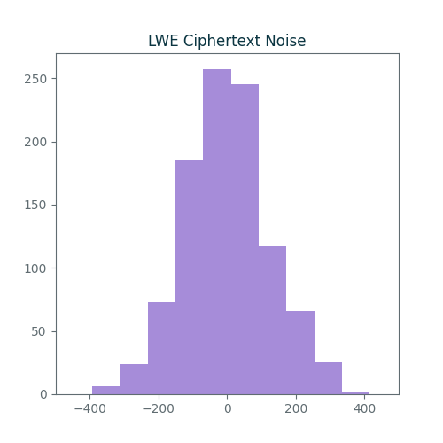
This matches our estimated standard deviation of $\sigma’=128$ pretty well.
Message Encoding
In the previous section we saw that when we decrypt a ciphertext with LWE we get the original message plus a small error. For some applications such as neural networks a small amount of error may be tolerable. An alternative approach is to restrict the set of possible messages so that a message $m$ can be recovered from $m+e$ by rounding to the nearest message in the restricted set.
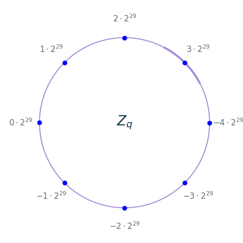
For the purposes of this post we will only need to distinguish between 8 different messages and so all of our messages will be of the form $m = i \cdot 2^{29}$ where $i \in \mathbb{Z}_8 = [-4, 4)$.
Here is a depiction of $\mathbb{Z}_q$ as a circle starting from $2^{31}$ in the “3 o’clock” position and going counter clockwise all the way around to $-2^{31}$. Note that $2^{31} = -2^{31}$ modulo $q=2^{32}$ which is why we are depicting $\mathbb{Z}_q$ as a closed circle. The eight messages $-4\cdot 2^{29}, \dots, 3\cdot 2^{29}$ are drawn as blue dots:
We will use the following encoding function to encode an integer $i \in \mathbb{Z}_8$ as an LWE plaintext in $\mathbb{Z}_q$ (i.e as a 32-bit integer):
\[\begin{align*} \mathrm{Encode}: \mathbb{Z}_8 &\rightarrow \mathbb{Z}_q \\ i &\mapsto i \cdot 2^{29} \end{align*}\]Similarly, we will use the following decoding function to convert a 32-bit LWE plaintext in $\mathbb{Z}_q$ back to an integer in $\mathbb{Z}_8$:
\[\begin{align*} \mathrm{Decode}: \mathbb{Z}_q & \rightarrow \mathbb{Z}_8 \\ m &\mapsto \lfloor m \cdot 2^{-29} \rceil \end{align*}\]where $\lfloor \cdot \rceil$ denotes rounding to the nearest integer. In terms of the image above, the decoding function maps a point on the circle to the nearest blue dot.
The thick segment of the circle depicts points whose distance from the message $m = 3 \cdot 2^{29}$ is less than $2^{28}$. Note that for the points in this segment, the closest blue dot is $m = 3\cdot 2^{29}$. In general, if $i \in \mathbb{Z}_8$ and $\vert e \vert < 2^{28}$ then
\[ \mathrm{Decode}(\mathrm{Encode}(i) + e) = i \]
In the previous section we saw that, using our standard LWE parameters, the distribution of LWE ciphertext errors has a standard deviation of around $2^7$ which is significantly less than $2^{28}$. This means that if $m = \mathrm{Encode}(i)$ and $L \in \mathrm{LWE}_{\mathbf{s}}(m)$ is an encryption of $m$ then we can decrypt $L$ and remove the noise by decoding:
\[\mathrm{Decode}(\mathrm{Dec}_{\mathbf{s}}(L)) = i\]In summary, if we only encrypt messages that are encodings of $\mathbb{Z}_8$ then we can use the decoding function to remove the noise from our decryption results.
Here is an implementation of the encoding and decoding functions:
def encode(i: int) -> np.int32:
    """Encode an integer in [-4, 4) as an int32"""
    return np.multiply(i, 1 << 29, dtype=np.int32)


def decode(i: np.int32) -> int:
    """Decode an int32 to an integer in the range [-4, 4) mod 8"""
    d = int(np.rint(i / (1 << 29)))
    return ((d + 4) % 8) - 4
def lwe_encode(i: int) -> LwePlaintext:
    """Encode an integer in [-4,4) as an LWE plaintext."""
    return LwePlaintext(utils.encode(i))


def lwe_decode(plaintext: LwePlaintext) -> int:
    """Decode an LWE plaintext to an integer in [-4,4) mod 8."""
    return utils.decode(plaintext.message)
In the following example we’ll use the encoding and decoding functions to encrypt a message and recover the exact message without noise after decryption.
LWE Message Encoding Example
key = lwe.generate_lwe_key(config.LWE_CONFIG)

# Encode the number 2 as an LWE plaintext
plaintext = lwe.lwe_encode(2)

# Encrypt the plaintext
ciphertext = lwe.lwe_encrypt(plaintext, key)

# Decrypt the ciphertext. The result will contain noise.
decrypted = lwe.lwe_decrypt(ciphertext, key)

# Decode the result of the decryption. The decoded decryption
# should be exactly equal to the initial message of 2.
decoded = lwe.lwe_decode(decrypted)

assert decoded == 2
Homomorphic Operations
In the next two sections we will show that the LWE scheme above is homomorphic under addition and multiplication by a plaintext.
More precisely, we will define a homomorphic addition function $\mathrm{CAdd}$ with the following signature:
\[ \mathrm{CAdd}: \mathrm{LWE}_{\mathbf{s}}(m_1) \times \mathrm{LWE}_{\mathbf{s}}(m_2) \rightarrow \mathrm{LWE}_{\mathbf{s}}(m_1 + m_2) \]
In other words, $\mathrm{CAdd}$ takes as input encryptions of $m_1$ and $m_2$ and outputs an encryption of $m_1 + m_2$.
Similarly, let $c \in \mathbb{Z}_q$ be an LWE plaintext. We will define a homomorphic “multiplication by $c$” function $\mathrm{PMul}$ with the signature:
\[ \mathrm{PMul}(c, \cdot): \mathrm{LWE}_{\mathbf{s}}(m) \rightarrow \mathrm{LWE}_{\mathbf{s}}(c \cdot m) \]
In other words, $\mathrm{PMul}$ takes as input a plaintext $c$ and an encryption of $m$ and outputs an encryption of $c\cdot m$.
Importantly, these homomorphic operations operate only on ciphertexts and do not receive the secret key $\mathbf{s}$ as an input.
We will add these operations to our library by implementing the following methods:
def lwe_add(
    ciphertext_left: LweCiphertext, ciphertext_right: LweCiphertext
) -> LweCiphertext:
    """Homomorphically add two LWE ciphertexts.

    If ciphertext_left is an encryption of m_left and ciphertext_right is
    an encryption of m_right then the output will be an encryption of
    m_left + m_right.
    """
    pass


def lwe_plaintext_multiply(c: int, ciphertext: LweCiphertext) -> LweCiphertext:
    """Homomorphically multiply an LWE ciphertext with a plaintext integer.

    If the ciphertext is an encryption of m then the output will be an
    encryption of c * m.
    """
    pass
Before showing how this works let’s take a minute to explain why this is both interesting and useful. Suppose a server hosts a simple linear regression model with weights $w_0$ and $w_1$ whose linear part is defined by:
\[ f(x_0, x_1) = w_0\cdot x_0 + w_1 \cdot x_1 \]
In addition, suppose you have two secret numbers $m_0$ and $m_1$ and you want to use an untrusted server to compute $f(m_0, m_1)$. Since the server is untrusted, you do not want to send $m_0$ or $m_1$. Instead you can leverage the homomorphic addition and multiplication methods above to run the following computation:
Homomorphic Operations Example
# Client side: Generate and encryption key and encrypt m_0 and m_1
key = lwe.generate_lwe_key(config.LWE_CONFIG)
ciphertext_0 = lwe.lwe_encrypt(m_0, key)
ciphertext_1 = lwe.lwe_encrypt(m_1, key)

# Send the ciphertexts to the untrusted server.

# Server side: Generate an encryption of
# f(m_0, m_1) = w_0*m_0 + w_1*m_1
ciphertext_result = lwe.lwe_add(
    lwe.lwe_plaintext_multiply(w_0, ciphertext_0),
    lwe.lwe_plaintext_multiply(w_1, ciphertext_1),
)

# The server sends ciphertext_f back to the client

# Client side: Decrypt ciphertext_result to obtain f(m_0, m_1)
result = lwe.lwe_decrypt(ciphertext_result, key)
Note that this example can easily be extended to general dot products between a vector of weights $\mathbf{w}$ and a vector of features $\mathbf{x}$ which is a core component of neural networks.
Homomorphic Addition
In this section we’ll implement the homomorphic addition function:
\[ \mathrm{CAdd}: \mathrm{LWE}_{\mathbf{s}}(m_1) \times \mathrm{LWE}_{\mathbf{s}}(m_2) \rightarrow \mathrm{LWE}_{\mathbf{s}}(m_1 + m_2) \]
Let $\mathbf{s}$ be a LWE key, let $m_1, m_2 \in \mathbb{Z}_q$ be two messages and let $L_1 = (\mathbf{a}_1, b_1)$ and $L_2 = (\mathbf{a}_2, b_2)$ be encryptions of $m_1$ and $m_2$ respectively.
By definition, $\mathrm{CAdd}(L_1, L_2)$ should be equal to a ciphertext $L_{\mathrm{sum}}$ that is an encryption of $m_1 + m_2$.
How can we obtain $L_{\mathrm{sum}}$ from the inputs $L_1$ and $L_2$?
It turns out that all we have to do is add the coefficients of $L_1$ and $L_2$:
\[ \mathrm{CAdd}(L_1, L_2) := (\mathbf{a}_1 + \mathbf{a}_2, b_1 + b_2) \]
To prove that $L_{\mathrm{sum}} = \mathrm{CAdd}(L_1, L_2)$ is indeed an encryption of $m_1 + m_2$, let’s decrypt it:
\[\begin{align*} \mathrm{Dec}_{\mathbf{s}}(L_{\mathrm{sum}}) &= \mathrm{Dec}_{\mathbf{s}}((\mathbf{a}_1 + \mathbf{a}_2, b_1 + b_2)) \\ &= (b_1 + b_2) - (\mathbf{a}_1 + \mathbf{a}_2) \cdot \mathbf{s} \\ &= (b_1 - \mathbf{a}_1 \cdot \mathbf{s}) + (b_2 - \mathbf{a}_2 \cdot \mathbf{s}) \\ &= \mathrm{Dec}_{\mathbf{s}}(L_1) + \mathrm{Dec}_{\mathbf{s}}(L_2) \\ &= (m_1 + e_1) + (m_2 + e_2)\\ &= (m_1 + m_2) + (e_1 + e_2) \end{align*}\]In summary:
\[\begin{equation}\label{eq:cadd-correctness} \mathrm{Dec}_{\mathbf{s}}(L_{\mathrm{sum}}) = (m_1 + m_2) + (e_1 + e_2) \end{equation}\]This proves that $L_{\mathrm{sum}}$ is an encryption of $m_1 + m_2$ with noise $e_1 + e_2$.
Later in this post we will also use the analogous homomorphic subtraction function $\mathrm{CSub}$:
\[ \mathrm{CSub}: \mathrm{LWE}_{\mathbf{s}}(m_1) \times \mathrm{LWE}_{\mathbf{s}}(m_2) \rightarrow \mathrm{LWE}_{\mathbf{s}}(m_1 - m_2) \]
Here are concrete implementations of $\mathrm{CAdd}$ and $\mathrm{CSub}$:
def lwe_add(
    ciphertext_left: LweCiphertext,
    ciphertext_right: LweCiphertext) -> LweCiphertext:
    """Homomorphic addition evaluation.

       If ciphertext_left is an encryption of m_left and ciphertext_right is
       an encryption of m_right then return an encryption of
       m_left + m_right.
    """
    return LweCiphertext(
        ciphertext_left.config,
        np.add(ciphertext_left.a, ciphertext_right.a, dtype=np.int32),
        np.add(ciphertext_left.b, ciphertext_right.b, dtype=np.int32))

def lwe_subtract(
    ciphertext_left: LweCiphertext,
    ciphertext_right: LweCiphertext) -> LweCiphertext:
    """Homomorphic subtraction evaluation.

       If ciphertext_left is an encryption of m_left and ciphertext_right is
       an encryption of m_right then return an encryption of
       m_left - m_right.
    """
    return LweCiphertext(
        ciphertext_left.config,
        np.subtract(ciphertext_left.a, ciphertext_right.a, dtype=np.int32),
        np.subtract(ciphertext_left.b, ciphertext_right.b, dtype=np.int32))
Here is an example of homomorphic addition:
key = lwe.generate_lwe_key(config.LWE_CONFIG)

# Encode the values 3 and -1 as LWE plaintexts
plaintext_a = lwe.lwe_encode(3)
plaintext_b = lwe.lwe_encode(-1)

# Encrypt both plaintexts
ciphertext_a = lwe.lwe_encrypt(plaintext_a, key)
ciphertext_b = lwe.lwe_encrypt(plaintext_b, key)

# Homomorphically add the ciphertexts.
ciphertext_sum = lwe.lwe_add(ciphertext_a, ciphertext_b)

# Decrypt the ciphertext_sum and then decode it. The result should
# be equal to 3 + (-1) = 2
decrypted = lwe.lwe_decrypt(ciphertext_sum, key)
decoded = lwe.lwe_decode(decrypted)
assert decoded == 2
Homomorphic Multiplication By Plaintext
In this section we’ll implement the homomorphic multiplication by plaintext function:
\[ \mathrm{PMul}(c, \cdot): \mathrm{LWE}_{\mathbf{s}}(m) \rightarrow \mathrm{LWE}_{\mathbf{s}}(c \cdot m) \]
Let $\mathbf{s}$ be a LWE key, let $c, m \in \mathbb{Z}_q$ be two messages and let $L = (\mathbf{a}, b)$ be an encryption of $m$.
By definition, $\mathrm{PMul}(c, L)$ should be equal to a ciphertext $L_{\mathrm{prod}}$ that is an encryption of $c \cdot m$.
Inspired by the previous section, we can attempt to implement $\mathrm{PMul}$ by element wise multiplication of the scalar $c$ with the vector $L = (\mathbf{a}, b)$:
\[ \mathrm{PMul}(c, L) := c \cdot L = (c \cdot \mathbf{a}, c \cdot b) \]
As before, we can verify that this is correct by decrypting $L_{\mathrm{prod}} = \mathrm{PMul}(c, L)$:
\[\begin{align*} \mathrm{Dec}_{\mathbf{s}}(L_{\mathrm{prod}}) &= \mathrm{Dec}_{\mathbf{s}}((c \cdot \mathbf{a}, c \cdot b)) \\ &= (c \cdot b) - (c \cdot \mathbf{a}) \cdot \mathbf{s} \\ &= c \cdot (b - \mathbf{a} \cdot \mathbf{s}) \\ &= c \cdot (m + e) \\ &= (c \cdot m) + (c \cdot e) \end{align*}\]This shows that the result of decrypting $L_{\mathrm{prod}}$ is the product $c \cdot m$ together with some noise that is equal to $c \cdot e$. If $c$ is small then the noise is small and so $\mathrm{PMul}(c, L)$ is a valid encryption of $c \cdot m$. We’ll analyze the noise more closely in the next section.
Here is an implementation of $\mathrm{PMul}$:
def lwe_plaintext_multiply(c: int, ciphertext: LweCiphertext) -> LweCiphertext:
    """Homomorphically multiply an LWE ciphertext with a plaintext integer."""
    return LweCiphertext(
        ciphertext.config,
        np.multiply(c, ciphertext.a, dtype=np.int32),
        np.multiply(c, ciphertext.b, dtype=np.int32),
    )
Noise Analysis
In this section we’ll analyze the effects of homomorphic operations on ciphertext noise.
Let $m_1$ and $m_2$ be LWE plaintexts. Let $L_i$ be an LWE encryption of $m_i$ with noise $e_i$. By equation \ref{eq:cadd-correctness}, $\mathrm{CAdd}(L_1, L_2)$ is an encryption of $m_1 + m_2$ with noise $e_1 + e_2$. This means that when we homomorphically add two ciphertexts, the noise in each of the inputs gets added to the result.
For example, let’s see what happens when we take an encryption of $0$ and homomorphically add it to itself 10 times. We’ll repeat the entire process 1000 times and plot the ciphertext error distribution before and after the homomorphic addition:
Homomorphic Addition Noise Analysis
key = lwe.generate_lwe_key(config.LWE_CONFIG)
plaintext_zero = lwe.LwePlaintext(0)

initial_errors = []
addition_errors = []

for _ in range(1000):
    # Encrypt the plaintext and record the ciphertext error.
    ciphertext_zero = lwe.lwe_encrypt(plaintext_zero, key)
    initial_errors.append(lwe.lwe_decrypt(ciphertext_zero, key).message)

    # Homomorphically add the ciphertext to itself 10 times.
    ciphertext_sum = ciphertext_zero
    for _ in range(10):
        ciphertext_sum = lwe.lwe_add(ciphertext_sum, ciphertext_zero)

    # Record the error of the ciphertext sum.
    addition_errors.append(lwe.lwe_decrypt(ciphertext_sum, key).message)
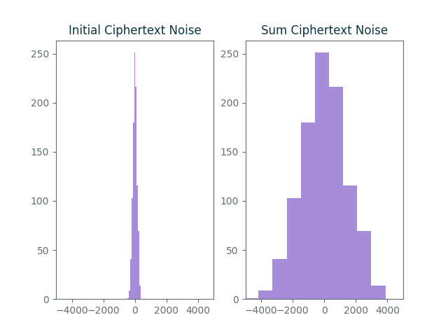
The graph on the left shows the distribution of initial_errors which records
the errors in the initial encryptions of $0$. The graph on the right shows the
distribution of addition_errors which contains the ciphertext errors after 10
homomorphic additions. As expected, the noise on the right is about 10 times
larger.
The maximum error in the graph on the right is around 5000 which is still significantly smaller than the maximal acceptable error of $2^{28}$. However, after $2^{20}$ homomorphic additions we’d eventually surpass that limit and no longer be able to accurately decode messages.
A major goal for the rest of this post is to develop a homomorphic operation whose output noise is independent of the input noise. This will make it possible to compose an arbitrary number of homomorphic operations, without running into the noise issue above.
Trivial Encryption
Let $m$ be an LWE plaintext and let $\mathbf{s}$ be an LWE encryption key. Consider the tuple:
\[L := (\mathbf{0}, m)\]where $\mathbf{0}$ is a length $n$ vector of zeroes. We claim that $L$ is a valid LWE encryption of $m$ with no noise. Indeed, the decryption of $L$ is exactly equal to $m$:
\[\mathrm{Dec}_{\mathbf{s}}(L) = m - \mathbf{0} \cdot \mathbf{s} = m\]The ciphertext $L$ is called the trivial encryption of $m$.
Here is our library implementation:
def lwe_trivial_ciphertext(plaintext: LwePlaintext, config: LweConfig):
    """Generate a trivial encryption of the plaintext."""
    return LweCiphertext(
        config=config,
        a=np.zeros(config.dimension, dtype=np.int32),
        b=plaintext.message,
    )
As an example of why this is useful, let $m_1$ be an LWE plaintext and let $L_2\in\mathrm{LWE}_{\mathbf{s}}(m_2)$ be an LWE encryption of $m_2$. How can we homomorphically add $m_1$ to $L_2$ to produce an encryption of $m_1 + m_2$?
In section Homomorphic Addition we implemented the function $\mathrm{CAdd}$ which homomorphically adds two LWE ciphertexts. We cannot directly apply $\mathrm{CAdd}$ since we are trying to add the plaintext $m_1$ to the ciphertext $L$. Instead, we can first convert $m_1$ to its trivial encryption $L_1$ and then compute $\mathrm{CAdd}(L_1, L_2)$.
Homomorphic NAND Revisited
In the previous section we introduced the LWE encryption scheme together with some basic homomorphic operations. This will allow us to refine our definition of the homomorphic NAND gate from section A Fully Homomorphic Nand Gate and give an overview of our implementation strategy.
Definition
In this section we’ll introduce an encoding of boolean values as LWE messages and precisely define the homomorphic NAND function.
We’ll use the $\mathrm{Encode}$ function from section Message Encoding to represent boolean values as LWE plaintexts. Specifically, we’ll represent $\mathrm{True}$ by $\mathrm{Encode}(2)$ and represent $\mathrm{False}$ by $\mathrm{Encode}(0)$.
Let $b_0$ and $b_1$ denote two booleans with the above representation. The homomorphic NAND gate $\mathrm{CNAND}$ has the signature:
\[\mathrm{CNAND}: \mathrm{LWE}_{\mathbf{s}}(b_0) \times \mathrm{LWE}_{\mathbf{s}}(b_1) \rightarrow \mathrm{LWE}_{\mathbf{s}}(\mathrm{NAND}(b_0, b_1))\]In other words, if $L_0 \in \mathrm{LWE}_{\mathbf{s}}(b_0)$ is an LWE encryption of $b_0$ and $L_1\in \mathrm{LWE}_{\mathbf{s}}(b_1)$ is an LWE encryption of $b_1$ then $\mathrm{CNAND}(L_0, L_1)$ is an LWE encryption of $\mathrm{NAND}(b_0, b_1)$.
Another important requirement for $\mathrm{CNAND}$ is that the noise of the output ciphertext $\mathrm{CNAND}(L_0, L_1)$ should be bounded and independent of the noise of the inputs $L_0$ and $L_1$. This property will make it possible to compose an arbitrary number of homomorphic NAND gates without suffering from the noise explosion issue that we saw in section Noise Analysis.
Here are the functions we’ll use to encode booleans as LWE plaintexts and to
decode plaintexts back to booleans. Note that we’re using the encode and
decode functions defined here.
def encode_bool(b: bool) -> np.int32:
    """Encode a bit as an int32."""
    return encode(2 * int(b))


def decode_bool(i: np.int32) -> bool:
    """Decode an int32 to a bool."""
    return bool(decode(i) / 2)
def lwe_encode_bool(b: bool) -> LwePlaintext:
    """Encode a boolean as an LWE plaintext."""
    return LwePlaintext(utils.encode_bool(b))


def lwe_decode_bool(plaintext: LwePlaintext) -> bool:
    """Decode an LWE plaintext to a boolean."""
    return utils.decode_bool(plaintext.message)
The signature of our homomorphic NAND function is:
def lwe_nand(
    lwe_ciphertext_left: lwe.LweCiphertext,
    lwe_ciphertext_right: lwe.LweCiphertext,
    bootstrap_key: bootstrap.BootstrapKey,
) -> lwe.LweCiphertext:
    """Homomorphically evaluate the NAND function.

    Suppose that lwe_ciphertext_left is an LWE encryption of
    lwe_encode_bool(b_left) and lwe_ciphertext_right is an LWE encryption
    lwe_encode_bool(b_right). Then the the output is an LWE encryption
    lwe_encode_bool(NAND(b_left, b_right)).
    """
    pass
As we’ll see later, bootstrap_key is a
public key that untrusted parties can use to homomorphically evaluate functions.
Here is an example:
# Generate a private LWE encryption key.
lwe_key = lwe.generate_lwe_key(config.LWE_CONFIG)

# Generate a public bootstrapping key.
gsw_key = gsw.convert_lwe_key_to_gsw(lwe_key, config.GSW_CONFIG)
bootstrap_key = bootstrap.generate_bootstrap_key(lwe_key, gsw_key)

# Encode two boolean values as LWE plaintexts.
plaintext_0 = lwe.lwe_encode_bool(False)
plaintext_1 = lwe.lwe_encode_bool(True)

# Encrypt the plaintexts.
ciphertext_0 = lwe.lwe_encrypt(plaintext_0, lwe_key)
ciphertext_1 = lwe.lwe_encrypt(plaintext_1, lwe_key)

# Homomorphically compute the NAND function on the inputs.
ciphertext_nand = nand.lwe_nand(
    ciphertext_0, ciphertext_1, bootstrap_key
)

# Decrypt the homomorphic NAND result with the LWE key.
plaintext_nand = lwe.lwe_decrypt(ciphertext_nand, lwe_key)

# Decode the LWE plaintext back to a bool.
boolean_nand = lwe.lwe_decode_bool(plaintext_nand)

# The result should be equal to NAND(False, True) = True
assert boolean_nand == True
Implementation Strategy
The remainder of this post will be dedicated to implementing lwe_nand. In this
section we’ll discuss our high level strategy.
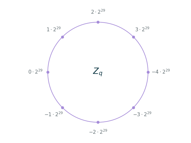
Recall that our encoding function $\mathrm{Encode}$ maps values from $\mathbb{Z}_8 = [-4, 4)$ to $\mathbb{Z}_q = [-2^{31}, 2^{31})$ and is defined by $\mathrm{Encode}(i) := i \cdot 2^{29}$:
We’ll start by expressing NAND in terms of elementary operations on $\mathbb{Z}_q$.
As before, we will identify $\mathrm{True}$ with $\mathrm{Encode}(2)$ and $\mathrm{False}$ with $\mathrm{Encode}(0)$. Let $b_0, b_1 \in \{\mathrm{Encode}(0), \mathrm{Encode}(2)\}$ be two boolean values and consider the expression:
\[F(b_0, b_1) = \mathrm{Encode}(-3) - b_0 - b_1 \]
In terms of the diagram above, we start at $\mathrm{Encode}(-3) = -3 \cdot 2^{29}$ and move two dots counter clockwise for each $b_i$ that is “true”. Here are the four possible values (modulo $q = 2^{32}$) that this expression can take:
| $b_0$ | $b_1$ | $F(b_0, b_1)$ |
|---|---|---|
| $\mathrm{Encode}(0)$ | $\mathrm{Encode}(0)$ | $\mathrm{Encode}(-3)$ |
| $\mathrm{Encode}(0)$ | $\mathrm{Encode}(2)$ | $\mathrm{Encode}(3)$ |
| $\mathrm{Encode}(2)$ | $\mathrm{Encode}(0)$ | $\mathrm{Encode}(3)$ |
| $\mathrm{Encode}(2)$ | $\mathrm{Encode}(2)$ | $\mathrm{Encode}(1)$ |
Note that $-2 \cdot 2^{29} < F(b_0, b_1) \leq 2 \cdot 2^{29}$ if and only if $b_0 = b_1 = \mathrm{Encode}(2)$. We can therefore upgrade $F(b_0, b_1)$ to a NAND function by composing it with the step function $\mathrm{Step}(x)$ which is defined on $\mathbb{Z}_q$ as follows:
\[\begin{equation}\label{def:step} \mathrm{Step}(x) = \begin{cases} 0 & -q/4 < x \leq q/4 \\ \mathrm{Encode}(2) & \mathrm{else} \end{cases} \end{equation}\]Here’s what happens when we apply $\mathrm{Step}(x)$ to $F(b_0, b_1)$:
| $b_0$ | $b_1$ | $F(b_0, b_1)$ | $\mathrm{Step}(F(b_0, b_1))$ |
|---|---|---|---|
| $\mathrm{Encode}(0)$ | $\mathrm{Encode}(0)$ | $\mathrm{Encode}(-3)$ | $\mathrm{Encode}(2)$ |
| $\mathrm{Encode}(0)$ | $\mathrm{Encode}(2)$ | $\mathrm{Encode}(3)$ | $\mathrm{Encode}(2)$ |
| $\mathrm{Encode}(2)$ | $\mathrm{Encode}(0)$ | $\mathrm{Encode}(3)$ | $\mathrm{Encode}(2)$ |
| $\mathrm{Encode}(2)$ | $\mathrm{Encode}(2)$ | $\mathrm{Encode}(1)$ | $\mathrm{Encode}(0)$ |
It is evident from the table that
\[\begin{align*} \mathrm{NAND}(b_0, b_1) &= \mathrm{Step}(F(b_0, b_1)) \\ &= \mathrm{Step}(\mathrm{Encode}(-3) - b_0 - b_1) \end{align*}\]In summary, we’ve expressed the NAND function in terms of two operations on $\mathbb{Z}_q$: subtraction and the step function.
In section Homomorphic Addition we already implemented a homomorphic subtraction function $\mathrm{CSub}$. Therefore, all that remains is to implement a homomorphic step function. In the remainder of this post we will develop the bootstrapping function $\mathrm{Bootstrap}$ which is essentially a homomorphic step function that also has bounded output noise.
We can then use $\mathrm{CSub}$ and $\mathrm{Boostrap}$ to implement $\mathrm{CNAND}$:
\[ \mathrm{CNAND}(L_0, L_1) = \mathrm{Bootstrap}( \mathrm{CSub}(\mathrm{CSub}(\mathrm{Encode}(-3), L_0), L_1) ) \]
Here is the python implementation:
import numpy as np

from tfhe import bootstrap, lwe


def lwe_nand(
    lwe_ciphertext_left: lwe.LweCiphertext,
    lwe_ciphertext_right: lwe.LweCiphertext,
    bootstrap_key: bootstrap.BootstrapKey,
) -> lwe.LweCiphertext:
    """Homomorphically evaluate the NAND function.

    Suppose that lwe_ciphertext_left is an LWE encryption of an encoding of the
    boolean b_left and lwe_ciphertext_right is an LWE encryption of an encoding
    of the boolean b_right. Then the the output is an LWE encryption of an encoding
    of NAND(b_left, b_right).
    """
    # Compute an LWE encryption of: encode(-3) - b_left - b_right
    # First create a trivial encryption of encode(-3)
    initial_lwe_ciphertext = lwe.lwe_trivial_ciphertext(
        plaintext=lwe.lwe_encode(-3),
        config=lwe_ciphertext_left.config,
    )

    # Homomorphically subtract lwe_ciphertext_left and lwe_ciphertext_right
    lwe_ciphertext = lwe.lwe_subtract(
        initial_lwe_ciphertext, lwe_ciphertext_left
    )
    lwe_ciphertext = lwe.lwe_subtract(
        test_lwe_ciphertext, lwe_ciphertext_right
    )

    # Bootstrap lwe_ciphertext to output encode_bool(False) or
    # encode_bool(True).
    return bootstrap.bootstrap(
        lwe_ciphertext, bootstrap_key, scale=utils.encode_bool(True)
    )
Bootstrapping
Definition
In the context of TFHE, the $\mathrm{Bootstrap}$ function is a homomorphic version of the $\mathrm{Step}$ function defined in equation \ref{def:step}.
More precisely, let $m \in \mathbb{Z}_q$ be an LWE message. The signature of $\mathrm{Bootstrap}$ is:
\[\mathrm{Bootstrap}: \mathrm{LWE}_{\mathbf{s}}(m) \rightarrow \mathrm{LWE}_{\mathbf{s}}(\mathrm{Step}(m))\]In other words, $\mathrm{Bootstrap}$ takes as input an LWE encryption of a message $m$ and outputs an LWE encryption of $\mathrm{Step}(m)$.
The other key property of $\mathrm{Bootstrap}$ is that the noise distribution of its output ciphertext is independent of the noise of the input. This property is what will allow us to compose an arbitrary number of homomorphic NAND functions without an explosion of the ciphertext noise.
Here is the declaration of the $\mathrm{Bootstrap}$ function:
def bootstrap(
    lwe_ciphertext: lwe.LweCiphertext,
    bootstrap_key: BootstrapKey,
    scale: np.int32,
) -> lwe.LweCiphertext:
    """Bootstrap the LWE ciphertext.

    Suppose that lwe_ciphertext is an encryption of the int32 i.
    If -2^30 < i <= 2^30 then return an LWE encryption of the scale argument.
    Otherwise return an LWE encryption of 0. In both cases the ciphertext noise
    will be bounded and independent of the lwe_ciphertext noise.
    """
    pass
The bootstrap_key argument will be explained
later in this post. The scale parameter is
the non zero output value of the step function. Our definition of
$\mathrm{Step}$ above corresponds to scale = utils.encode(2).
Noise Properties
As mentioned in the previous section, a key property of the bootstrap function is that it has bounded output noise. In this section we’ll explore this property in more detail through an example.
Let $m_0=\mathrm{Encode}(0)$ and $m_1 = \mathrm{Encode}(3)$ be two LWE messages. Let $L_0 = \mathrm{Encrypt}_{\mathbf{s}}(m_0)$ be an encryption of $m_0$ and $L_1 = \mathrm{Encrypt}_{\mathbf{s}}(m_1)$ and encryption of $m_1$.
Suppose we homomorphically multiply $L_0$ by $2^{20}$ and add the result to $L_1$:
\[ L = \mathrm{CAdd}(L_1, \mathrm{PMul}(2^{20}, L_0)) \]
As we saw in section Homomorphic Multiplication By Plaintext, $\mathrm{PMul}(2^{20}, L_0)$ is an encryption of $2^{20} \cdot 0 = 0$. Therefore, $L$ is an encryption of $\mathrm{Encode}(3) + 0 = \mathrm{Encode}(3)$. Furthermore, as we saw in section Noise Analysis, we the expect noise distribution of $L$ to roughly have a standard deviation of $2^{20} \cdot 2^7 = 2^{27}$.
The following program computes the ciphertexts $L$ and $\mathrm{Bootstrap}(L)$ 1000 times so that we can compare the distributions of the decryptions $\mathrm{Dec}_{\mathbf{s}}(L)$ and $\mathrm{Dec}_{\mathbf{s}}(\mathrm{Bootstrap}(L))$:
Bootstrap Noise Distribution
from tfhe import bootstrap, gsw, lwe, utils

lwe_key = lwe.generate_lwe_key(config.LWE_CONFIG)
gsw_key = gsw.convert_lwe_key_to_gsw(lwe_key, config.GSW_CONFIG)
bootstrap_key = bootstrap.generate_bootstrap_key(lwe_key, gsw_key)

plaintext_0 = lwe.lwe_encode(0)
plaintext_3 = lwe.lwe_encode(3)

decryptions = []
bootstrap_decryptions = []

for _ in range(1000):
    ciphertext_0 = lwe.lwe_encrypt(plaintext_0, lwe_key)
    ciphertext_3 = lwe.lwe_encrypt(plaintext_3, lwe_key)

    ciphertext = lwe.lwe_add(
        ciphertext_3, lwe.lwe_plaintext_multiply(2**20, ciphertext_0))

    bootstrap_ciphertext = bootstrap.bootstrap(
        ciphertext, bootstrap_key, scale=utils.encode(2)
    )

    decryptions.append(lwe.lwe_decrypt(ciphertext, lwe_key).message)
    bootstrap_decryptions.append(
        lwe.lwe_decrypt(bootstrap_ciphertext, lwe_key).message)
Here is a comparison of the array decryptions which holds decryptions of $L$
and the array bootstrap_decryptions which holds decryptions of
$\mathrm{Bootstrap}(L)$:
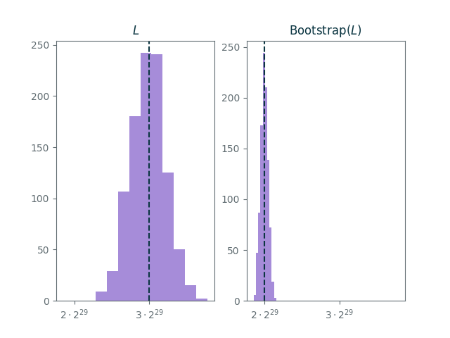
As expected, the distribution of decryptions of $L$ is centered at $\mathrm{Encode}(3) = 3 \cdot 2^{29}$ with a standard deviation of $2^{27}$.
After bootstrapping, the distribution of decryptions is centered at
\[ \mathrm{Step}(\mathrm{Encode}(3)) = \mathrm{Encode}(2) = 2 \cdot 2^{29} \]
Furthermore, the distribution clearly is less noisy after bootstrapping. Indeed, the standard deviation of $\mathrm{Bootstrap}(L)$ is $2^{25}$ which is less than the standard deviation of $L$!
Implementation Strategy
The rest of this post will build towards an implementation of $\mathrm{Bootstrap}$. The implementation will rely on an extension of LWE called Ring LWE where messages can be polynomials rather than scalars. The general idea is that we will express $\mathrm{Step}$ in terms of polynomial multiplication, and then use homomorphic polynomial multiplication to derive a homomorphic version of $\mathrm{Step}$.
If you prefer to get a high level picture of the implementation before diving into all the details, then it would make sense to start with the following sections:
Ring LWE
Introduction
Ring LWE (RLWE) is a variation of LWE in which messages are polynomials rather than scalars. As mentioned in the previous section, the RLWE encryption scheme will be an important ingredient in our bootstrapping implementation.
In the next section we’ll define the message space of RLWE more precisely. Then we’ll define the RLWE encryption scheme.
Negacyclic Polynomials
The message space of the RLWE scheme is the ring of polynomials
\[ \mathbb{Z}_q[x] / (x^n + 1) \]
In this section we will describe this polynomial ring.
First, $\mathbb{Z}_q[x]$ denotes the ring of polynomials with coefficients in $\mathbb{Z}_q$. As before, we will assume that $q=2^{32}$ and identify $\mathbb{Z}_q$ with signed 32 bit integers. In this context $\mathbb{Z}_q[x]$ denotes the ring of polynomials integer coefficients.
Here is an example of an element in $\mathbb{Z}_q[x]$:
\[ f(x) = 1 + 2x - 5x^3 \]
We call $\mathbb{Z}_q[x]$ a Ring because we can add and multiply elements. For example, if $f(x) = 1 + 2x - 5x^3$ and $g(x) = 1 + x$ then $f(x) + g(x) = 2 + 3x - 5x^3$ and $f(x)\cdot g(x) = 1 + 3x + 2x^2 - 5x^3 - 5x^4$.
The highest power of $x$ in a polynomial is called the degree. For example, the degree of $f(x)$ is $3$ and the degree of $g(x)$ is $1$. Polynomials in $\mathbb{Z}_q[x]$ can have arbitrarily high degrees.
We now turn to the ring $\mathbb{Z}_q[x] / (x^n + 1)$. The denominator $x^n+1$ plays a similar role to the denominator in $\mathbb{Z}_q = \mathbb{Z} / q\mathbb{Z}$. Two integers are considered to be equal modulo $q$ if they differ by a multiple of $q$. Similarly, two polynomials are considered to be equal modulo $x^n + 1$ if they differ by a multiple of $x^n + 1$.
$\mathbb{Z}_q[x] / (x^n + 1)$ is defined to be the ring of polynomials modulo $x^n + 1$.
As an important special case, $x^n = -1\ (\mathrm{mod}\ x^n + 1)$. Therefore, if we are given a polynomial with a degree larger than $n$, we can find it’s representative modulo $x^n + 1$ by replacing $x^n$ with $-1$ as many times as necessary. For example, if $n=4$ then we have the following equivalences modulo $x^4 + 1$:
\[\begin{align*} x^4 &= -1\ (\mathrm{mod}\ x^4 + 1) \\ 1 + x^5 &= 1 + x \cdot x^4 = 1 - x \ (\mathrm{mod}\ x^4 + 1) \\ x^2 + x^8 &= x^2 + x^4 \cdot x^4 = x^2 + (- 1 \cdot -1) = 1 + x^2 \ (\mathrm{mod}\ x^4 + 1) \end{align*}\]Note that as monomials reach $x^4$ they loop back to $1$ but with a negative sign. For this reason polynomials of this form are sometimes called negacyclic.
Now let’s see an example of multiplication in $\mathbb{Z}_q[x] / (x^4 + 1)$. Let $f(x) = 1 + x^3$ and $g(x) = x$ be elements of $\mathbb{Z}_q[x] / (x^4 + 1)$. Their product is:
\[ f(x) \cdot g(x) = x + x^4 = x - 1 = -1 + x\ (\mathrm{mod}\ x^4 + 1) \]
Here is some negacyclic polynomial code that will be used later:
import numpy as np
import dataclasses


@dataclasses.dataclass
class Polynomial:
    """A polynomial in the ring Z_q[x] / (x^N + 1)"""
    N: int
    coeff: np.ndarray # Polynomial coefficients f_0, f_1, ..., f_{N-1}


def polynomial_constant_multiply(c: int, p: Polynomial) -> Polynomial:
    return Polynomial(N=p.N, coeff=np.multiply(c, p.coeff, dtype=np.int32))


def polynomial_multiply(p1: Polynomial, p2: Polynomial) -> Polynomial:
    """Multiply two negacyclic polynomials.

    Note that this is not an optimal implementation.
    See
    https://www.jeremykun.com/2022/12/09/negacyclic-polynomial-multiplication/
    for a more efficient version which uses FFTs.
    """
    N = p1.N

    # Multiply and pad the result to have length 2N-1.
    # Note that the polymul function expects the coefficients to be from highest
    # to lowest degree so we reverse our coefficients before and after using it.
    prod = np.polymul(p1.coeff[::-1], p2.coeff[::-1])[::-1]
    prod_padded = np.zeros(2 * N - 1, dtype=np.int32)
    prod_padded[: len(prod)] = prod

    # Use the relation x^N = -1 to obtain a polynomial of degree N-1
    result = prod_padded[:N]
    result[:-1] -= prod_padded[N:]
    return Polynomial(N=N, coeff=result)


def polynomial_add(p1: Polynomial, p2: Polynomial) -> Polynomial:
    return Polynomial(N=p1.N, coeff=np.add(p1.coeff, p2.coeff, dtype=np.int32))


def polynomial_subtract(p1: Polynomial, p2: Polynomial) -> Polynomial:
    return Polynomial(
        N=p1.N, coeff=np.subtract(p1.coeff, p2.coeff, dtype=np.int32)
    )


def zero_polynomial(N: int) -> Polynomial:
    return Polynomial(N=N, coeff=np.zeros(N, dtype=np.int32))


def build_monomial(c: int, i: int, N: int) -> Polynomial:
    """Build a monomial c*x^i in the ring Z[x]/(x^N + 1)"""
    coeff = np.zeros(N, dtype=np.int32)

    # Find k such that: 0 <= i + k*N < N
    i_mod_N = i % N
    k = (i_mod_N - i) // N

    # If k is odd then the monomial picks up a negative sign since:
    # x^i = (-1)^k * x^(i + k*N) = (-1)^k * x^(i % N)
    sign = 1 if k % 2 == 0 else -1

    coeff[i_mod_N] = sign * c
    return Polynomial(N=N, coeff=coeff)
The RLWE Encryption Scheme
In this section we will define the RLWE Encryption Scheme which is very similar to the LWE encryption scheme but with messages in $\mathbb{Z}_q[x] / (x^n + 1)$ rather than $\mathbb{Z}_q$.
A secret key in RLWE is a polynomial in $\mathbb{Z}_q[x] / (x^n + 1)$ with random binary coefficients. For example, if $n=4$ then a secret key may look like:
\[s(x) = 1 + 0\cdot x + 1\cdot x^2 + 1\cdot x^3 = 1 + x^2 + x^3\]To encrypt a message $m(x) \in \mathbb{Z}_q[x] / (x^n + 1)$ with the secret key $s(x)$ we first sample a polynomial $a(x)\in \mathbb{Z}_q[x]$ with uniformly random coefficients in $\mathbb{Z}_q$ and an error polynomial $e(x)\in \mathbb{Z}_q[x]$ with small error coefficients sampled from $\mathcal{N}_q$. The encryption of $m(x)$ by $s(x)$ is then given by the pair:
\[\mathrm{Enc}^{\mathrm{RLWE}}_{s(x)}(m(x)) = (a(x), a(x)\cdot s(x) + m(x) + e(x))\]To decrypt a ciphertext $(a(x), b(x))$ we compute:
\[\mathrm{Dec}^{\mathrm{RLWE}}_{s(x)}((a(x), b(x))) = b(x) - a(x)\cdot s(x) = m(x) + e(x)\]Similarly to LWE, the encryption function is not deterministic and so each message has many valid encryptions. The set of valid encryptions of a message $m(x)$ with the key $s(x)$ will be denoted $\mathrm{RLWE}_{s(x)}(m(x))$.
Here is our implementation of the RLWE scheme:
import dataclasses

import numpy as np

from tfhe import lwe, polynomial, utils
from tfhe.polynomial import Polynomial


@dataclasses.dataclass
class RlweConfig:
    degree: int  # Messages will be in the space Z[X]/(x^degree + 1)
    noise_std: float  # The std of the noise added during encryption.


@dataclasses.dataclass
class RlweEncryptionKey:
    config: RlweConfig
    key: Polynomial


@dataclasses.dataclass
class RlwePlaintext:
    config: RlweConfig
    message: Polynomial


@dataclasses.dataclass
class RlweCiphertext:
    config: RlweConfig
    a: Polynomial
    b: Polynomial


def generate_rlwe_key(config: RlweConfig) -> RlweEncryptionKey:
    return RlweEncryptionKey(
        config=config,
        key=Polynomial(
            N=config.degree,
            coeff=np.random.randint(
                low=0, high=2, size=config.degree, dtype=np.int32
            ),
        ),
    )

def rlwe_encrypt(
    plaintext: RlwePlaintext, key: RlweEncryptionKey
) -> RlweCiphertext:
    a = Polynomial(
        N=key.config.degree,
        coeff=utils.uniform_sample_int32(size=key.config.degree),
    )
    noise = Polynomial(
        N=key.config.degree,
        coeff=utils.gaussian_sample_int32(
            std=key.config.noise_std, size=key.config.degree
        ),
    )

    b = polynomial.polynomial_add(
        polynomial.polynomial_multiply(a, key.key), plaintext.message
    )
    b = polynomial.polynomial_add(b, noise)

    return RlweCiphertext(config=key.config, a=a, b=b)


def rlwe_decrypt(
    ciphertext: RlweCiphertext, key: RlweEncryptionKey
) -> RlwePlaintext:
    message = polynomial.polynomial_subtract(
        ciphertext.b, polynomial.polynomial_multiply(ciphertext.a, key.key)
    )
    return RlwePlaintext(config=key.config, message=message)
We’ll use the following RLWE parameters in this post:
RLWE_CONFIG = rlwe.RlweConfig(degree=1024, noise_std=2 ** (-24))
Message Encoding
As with LWE, after decrypting a ciphertext $m(x)\in\mathrm{RLWE}_{s(x)}(m(x))$ we get the original message $m(x)$ together with a small amount of noise $e(x)$. To achieve noiseless decryptions we’ll extend the $\mathrm{Encode}$ and $\mathrm{Decode}$ functions from Message Encoding to polynomials by encoding and decoding each individual coefficient.
The extended $\mathrm{Encode}$ function encodes a polynomial with coefficients in $\mathbb{Z}_8$ as a polynomial with coefficients in $\mathbb{Z}_q$:
\[\begin{align*} \mathrm{Encode}: \mathbb{Z}_8[x]/(x^N+1) &\rightarrow \mathbb{Z}_q[x]/(x^N+1) \\ a_0 + a_1x + \dots a_{n-1}x^{n-1} &\mapsto \mathrm{Encode}(a_0) + \mathrm{Encode}(a_1)x + \dots \mathrm{Encode}(a_{n-1})x^{n-1} \end{align*}\]Similarly, the extended $\mathrm{Decode}$ function will decode a polynomial with coefficients in $\mathrm{Z}_q$ to a polynomial with coefficients in $\mathrm{Z}_8$:
\[\begin{align*} \mathrm{Decode}: \mathbb{Z}_q[x]/(x^N+1) &\rightarrow \mathbb{Z}_8[x]/(x^N+1) \\ a_0 + a_1x + \dots a_{n-1}x^{n-1} &\mapsto \mathrm{Decode}(a_0) + \mathrm{Decode}(a_1)x + \dots \mathrm{Decode}(a_{n-1})x^{n-1} \end{align*}\]Just like with LWE, we’ll restrict our message space to encodings of $\mathbb{Z}_8[x]/(x^N+1)$. We can then apply $\mathrm{Decode}$ to remove the decryption error $e(x)$ as long as the absolute values of the coefficients of $e(x)$ are all less than $2^{28}$
Here is an implementation of the encoding and decoding functions for RLWE messages:
def rlwe_encode(p: Polynomial, config: RlweConfig) -> RlwePlaintext:
    """Encode a polynomial with coefficients in [-4, 4) as an RLWE plaintext."""
    encode_coeff = np.array([utils.encode(i) for i in p.coeff])
    return RlwePlaintext(
        config=config, message=polynomial.Polynomial(N=p.N, coeff=encode_coeff)
    )


def rlwe_decode(plaintext: RlwePlaintext) -> Polynomial:
    """Decode an RLWE plaintext to a polynomial with coefficients in [-4, 4) mod 8."""
    decode_coeff = np.array([utils.decode(i) for i in plaintext.message.coeff])
    return Polynomial(N=plaintext.message.N, coeff=decode_coeff)
Here is an example of using the RLWE encryption scheme with the above encoding:
RLWE Message Encoding Example
key = rlwe.generate_rlwe_key(config.RLWE_CONFIG)

# p(x) = 2x^3
p = polynomial.build_monomial(c=2, i=3, N=config.RLWE_CONFIG.degree)

# Encode the polynomial p(x) as an RLWE plaintext.
plaintext = rlwe.rlwe_encode(p, config)

# Encrypt the plaintext with the key.
ciphertext = rlwe.rlwe_encrypt(plaintext, key)

# Decrypt the ciphertext.
decrypted = rlwe.rlwe_decrypt(ciphertext, key)

# Decode the decrypted message to remove the noise.
decoded = rlwe.rlwe_decode(decrypted)

# The final decoded result should be equal to the original polynomial p.
assert np.all(decoded.coeff == p.coeff)
Homomorphic Addition
In this section we’ll develop the RLWE analog of LWE Homomorphic Addition.
Let $s(x)$ be an RLWE encryption key and let $f_1(x), f_2(x) \in \mathbb{Z}_q[x] / (x^n + 1)$ be RLWE plaintexts. The signature of the homomorphic addition function $\mathrm{CAdd}$ is:
\[\mathrm{CAdd}: \mathrm{RLWE}_{s(x)}(f_1(x)) \times \mathrm{RLWE}_{s(x)}(f_2(x)) \rightarrow \mathrm{RLWE}_{s(x)}(f_1(x) + f_2(x))\]In other words, $\mathrm{CAdd}$ takes an input RLWE encryptions of $f_1(x)$ and $f_2(x)$ and outputs an RLWE encryption of $f_1(x) + f_2(x)$.
Similarly to LWE Homomorphic Addition, we can implement $\mathrm{CAdd}$ for the RLWE scheme by adding the input ciphertexts element-wise:
\[\mathrm{CAdd}((a_1(x), b_1(x)), (a_2(x), b_2(x))) := (a_1(x) + a_2(x), b_1(x) + b_2(x))\]The RLWE version of the homomorphic subtraction function $\mathrm{CSub}$ is analogous.
Here is the corresponding code:
def rlwe_add(
    ciphertext_left: RlweCiphertext, ciphertext_right: RlweCiphertext
) -> RlweCiphertext:
    """Homomorphically add two RLWE ciphertexts."""
    return RlweCiphertext(
        ciphertext_left.config,
        polynomial.polynomial_add(ciphertext_left.a, ciphertext_right.a),
        polynomial.polynomial_add(ciphertext_left.b, ciphertext_right.b),
    )


def rlwe_subtract(
    ciphertext_left: RlweCiphertext, ciphertext_right: RlweCiphertext
) -> RlweCiphertext:
    """Homomorphically subtract two RLWE ciphertexts."""
    return RlweCiphertext(
        ciphertext_left.config,
        polynomial.polynomial_subtract(ciphertext_left.a, ciphertext_right.a),
        polynomial.polynomial_subtract(ciphertext_left.b, ciphertext_right.b),
    )
Homomorphic Multiplication By Plaintext
In this section we’ll develop the RLWE analog of LWE Homomorphic Multiplication By Plaintext.
Let $s(x)$ be an RLWE encryption key and let $c(x), f(x) \in \mathbb{Z}_q[x] / (x^n + 1)$ be RLWE plaintexts. The signature of the homomorphic multiplication by plaintext function $\mathrm{PMul}$ is:
\[\mathrm{PMul}(c(x), \cdot): \mathrm{RLWE}_{s(x)}(f(x)) \rightarrow \mathrm{RLWE}_{s(x)}(c(x) \cdot f(x))\]Let $R = (a(x), b(x)) \in \mathrm{RLWE}_{s(x)}(f(x))$ be an RLWE encryption of $f(x)$. Similarly to LWE Homomorphic Multiplication By Plaintext, we can implement $\mathrm{PMul}$ for the RLWE scheme by multiplying $c(x)$ with the vector $R$:
\[\mathrm{PMul}(c(x), (a(x), b(x))) := c(x) \cdot R = (c(x) \cdot a(x), c(x) \cdot b(x))\]Just like in the LWE case, $\mathrm{PMul}(c(x), R)$ is a valid RLWE encryption of $c(x) \cdot f(x)$ under the condition that the coefficients of $c(x)$ are small.
Here is an implementation:
def rlwe_plaintext_multiply(
    c: RlwePlaintext, ciphertext: RlweCiphertext
) -> RlweCiphertext:
    """Homomorphically multiply an RLWE ciphertext by a plaintext polynomial."""
    return RlweCiphertext(
        ciphertext.config,
        polynomial.polynomial_multiply(c.message, ciphertext.a),
        polynomial.polynomial_multiply(c.message, ciphertext.b),
    )
And here is an example:
key = rlwe.generate_rlwe_key(config.RLWE_CONFIG)

# c(x) = x, m(x) = 2x^2
c = polynomial.build_monomial(1, 1, N=config.RLWE_CONFIG.degree)
m = polynomial.build_monomial(2, 2, N=config.RLWE_CONFIG.degree)

# Convert c(x) into an RLWE plaintext without encoding. Note that encoding is
# not necessary since c(x) will not be encrypted.
c_plaintext = rlwe.RlwePlaintext(config=config.RLWE_CONFIG, message=c)

# Encode m(x) as an RLWE plaintext.
m_plaintext = rlwe.rlwe_encode(m, config)

# Encrypt m(x)
m_ciphertext = rlwe.rlwe_encrypt(m_plaintext, key)

# Homomorphically multiply the encryption of m(x) with c(x)
cm_ciphertext = rlwe.rlwe_plaintext_multiply(c_plaintext, m_ciphertext)

# Decrypt the product.
cm_decrypted = rlwe.rlwe_decrypt(cm_ciphertext, key)

# Decode the result.
cm_decoded = rlwe.rlwe_decode(cm_decrypted)

# The decoded result should be equal to c(x)*m(x) = 2x^3
assert np.all(cm_decoded.coeff == polynomial.polynomial_multiply(c, m))
Trivial Encryption
In this section we’ll define the RLWE analog of LWE Trivial Encryption
Let $f(x)$ be an RLWE plaintext. The trivial encryption of $f(x)$ is defined to be:
\[R = (0, f(x))\]As in the LWE case, it is easy to verify that this is a valid RLWE encryption of $f(x)$ with zero noise.
Here is an implementation:
def rlwe_trivial_ciphertext(
    f: Polynomial, config: RlweConfig
) -> RlweCiphertext:
    """Generate a trivial encryption of the plaintext."""
    if f.N != config.degree:
        raise ValueError(
            f"The degree of f ({f.N}) does not match the config degree ({config.degree}) "
        )

    return RlweCiphertext(
        config=config,
        a=polynomial.zero_polynomial(config.degree),
        b=f,
    )
LWE To RLWE Keys
Recall from section An LWE Based Encryption Scheme that LWE encryption keys are length $n$ vectors
\[\mathbf{s} = (s_0,\dots,s_{n-1})\]where $s_i \in {0, 1}$.
As we just saw, RLWE encryption keys are degree $N$ polynomials
\[s(x) = s_0 + s_1\cdot x + \dots + s_{N-1}\cdot x^{N-1}\]where $s_i \in {0, 1}$ as well.
In this post, we’ll be using the parameters $n = N = 1024$. Therefore, we can convert an LWE key $\mathbf{s}$ to an RLWE key $s(x)$ by forming a polynomial from the coefficients of $\mathbf{s}$.
def convert_lwe_key_to_rlwe(lwe_key: lwe.LweEncryptionKey) -> RlweEncryptionKey:
    rlwe_config = RlweConfig(
        degree=lwe_key.config.dimension, noise_std=lwe_key.config.noise_std
    )
    return RlweEncryptionKey(
        config=rlwe_config,
        key=Polynomial(N=rlwe_config.degree, coeff=lwe_key.key),
    )
The ability to convert LWE keys to RLWE keys will come in handy in sections Blind Rotate and Sample Extraction where we’ll implement homomorphic operations that combine both LWE and RLWE ciphertexts.
A Homomorphic Multiplexer
Introduction
The Multiplexer gate has three inputs: a selector bit $b$ and two lines $l_0$ and $l_1$. The output is defined by:
\[\mathrm{Mux}(b, l_0, l_1) = \begin{cases} l_0 & \mathrm{if}\ b = 0 \\ l_1 & \mathrm{if}\ b = 1 \end{cases}\]In other words, the multiplexer outputs one of the two input lines depending on the selector bit.
Our implementation of bootstrapping will require a homomorphic multiplexer $\mathrm{CMux}$. The $\mathrm{CMux}$ function also has three inputs: An encrypted selector bit $\mathrm{Enc}(b)$ and RLWE encryptions of the two lines $l_0(x)$ and $l_1(x)$. The output is an RLWE encryption of $\mathrm{Mux}(b, l_0(x), l_1(x))$:
\[\mathrm{CMux}: \mathrm{Enc}_{s(x)}(b) \times \mathrm{RLWE}_{s(x)}(l_0(x)) \times \mathrm{RLWE}_{s(x)}(l_1(x)) \rightarrow \mathrm{RLWE}_{s(x)}(\mathrm{Mux}(b, l_0(x), l_1(x)))\]Note that, for reasons that will soon become clear, we have not yet specified the encryption scheme used to encrypt $b$.
The goal of this section is to implement $\mathrm{CMux}$.
The first step is to note that we can express the standard $\mathrm{Mux}$ function in terms of addition, subtraction and multiplication:
\begin{equation}\label{eq:mux} \mathrm{Mux}(b, l_0, l_1) = b \cdot (l_1 - l_0) + l_0 \end{equation}
Therefore, all we need to do to implement $\mathrm{CMux}$ is to homomorphically evaluate the right hand side of equation \ref{eq:mux}. In section Homomorphic Addition we saw how to homomorphically evaluate addition and subtraction of RLWE ciphertexts. In section Homomorphic Multiplication By Plaintext we saw how to homomorphically multiply an RLWE ciphertext by an RLWE plaintext. This is not quite enough to homomorphically evaluate the multiplication in equation \ref{eq:mux} since both the selection bit $b$ and the lines $l_0$ and $l_1$ need to be encrypted.
In the next section we will introduce the GSW encryption scheme and implement homomorphic multiplication between a GSW ciphertext and an RLWE ciphertext:
\[\mathrm{CMul} : \mathrm{GSW}_{s(x)}(f_1(x)) \times \mathrm{RLWE}_{s(x)}(f_2(x)) \rightarrow \mathrm{RLWE}_{s(x)}(f_1(x) \cdot f_2(x))\]We’ll use the GSW scheme to encrypt the selector bit, and so we can update the signature of $\mathrm{CMux}$ to:
\[\mathrm{CMux}: \mathrm{GSW}_{s(x)}(b) \times \mathrm{RLWE}_{s(x)}(l_0(x)) \times \mathrm{RLWE}_{s(x)}(l_1(x)) \rightarrow \mathrm{RLWE}_{s(x)}(\mathrm{Mux}(b, l_0(x), l_1(x)))\]We can implement this version of $\mathrm{CMux}$ using $\mathrm{CAdd}$, $\mathrm{CSub}$ and $\mathrm{CMul}$ to homomorphically evaluate the right hand side of equation \ref{eq:mux}. More precisely, let $G \in \mathrm{GSW}_{s(x)}(b)$ be a GSW encryption of $b$ and let $R_i \in \mathrm{RLWE}_{s(x)}(l_i(x))$ be RLWE encryptions of $l_0(x)$ and $l_1(x)$. Then:
\[\mathrm{CMux}(B, R_0, R_1) = \mathrm{CAdd}(\mathrm{CMul}(B, \mathrm{CSub}(R_1, R_0)), R_0)\]Here is an implementation of $\mathrm{CMux}$ which builds on the GSW encryption scheme and the $\mathrm{CMul}$ function that we’ll explore in the next section.
def cmux(
    gsw_ciphertext: GswCiphertext,
    rlwe_ciphertext_0: rlwe.RlweCiphertext,
    rlwe_ciphertext_1: rlwe.RlweCiphertext,
) -> rlwe.RlweCiphertext:
    """Homomorphically evaluate the multiplexer function.

    Suppose that rlwe_ciphertext_0 is an encryption of l_0 and rlwe_ciphertext_1
    is an encryption of l_1. If gsw_ciphertext is a GSW encryption of 0, then
    the output will be an RLWE encryption of l_0. Otherwise, the output will be
    an RLWE encryption of l_1.
    """
    return rlwe.rlwe_add(
        gsw_multiply(
            gsw_ciphertext,
            rlwe.rlwe_subtract(rlwe_ciphertext_1, rlwe_ciphertext_0),
        ),
        rlwe_ciphertext_0,
    )
Here is an example:
rlwe_config = config.RLWE_CONFIG
gsw_config = config.GSW_CONFIG

# Generate an RLWE key and convert it to a GSW key.
rlwe_key = rlwe.generate_rlwe_key(rlwe_config)
gsw_key = gsw.convert_rlwe_key_to_gsw(rlwe_key, gsw_config)

# The selector bit is b=1
selector = polynomial.build_monomial(c=1, i=0, N=rlwe_config.degree)

# The lines are: l_0(x) = x, l_1(x) = 2x
line_0 = polynomial.build_monomial(c=1, i=1, N=rlwe_config.degree)
line_1 = polynomial.build_monomial(c=2, i=1, N=rlwe_config.degree)

# Create a GSW plaintext from the selector bit.
selector_plaintext = gsw.GswPlaintext(config=gsw_config, message=selector)

# Create RLWE plaintexts by encoding the lines.
line_0_plaintext = rlwe.rlwe_encode(line_0, rlwe_config)
line_1_plaintext = rlwe.rlwe_encode(line_1, rlwe_config)

# Encrypt the selector bit with GSW and the lines with RLWE.
selector_ciphertext = gsw.gsw_encrypt(selector_plaintext, gsw_key)
line_0_ciphertext = rlwe.rlwe_encrypt(line_0_plaintext, rlwe_key)
line_1_ciphertext = rlwe.rlwe_encrypt(line_1_plaintext, rlwe_key)

# Apply the CMux function to homomorphically evaluate Mux(b, l_0, l_1).
# This can be done on an untrusted server since all the inputs are encrypted.
cmux_ciphertext = gsw.cmux(
    selector_ciphertext, line_0_ciphertext, line_1_ciphertext)

# Decrypt the cmux result using the RLWE key.
cmux_decrypted = rlwe.rlwe_decrypt(cmux_ciphertext, rlwe_key)

# Decode the decrypted result.
cmux_decoded = rlwe.rlwe_decode(cmux_decrypted)

# Since the selector bit was b=1, the cmux result should be equal to line_1.
assert np.all(cmux_decoded.coeff == line_1.coeff)
The GSW Encryption Scheme
The GSW encryption scheme was proposed in 2013 by Gentry, Sahai and Waters. In this section we’ll define GSW encryption and implement homomorphic multiplication between a GSW ciphertext and an RLWE ciphertext:
\[\mathrm{CMul} : \mathrm{GSW}_{s(x)}(f_1(x)) \times \mathrm{RLWE}_{s(x)}(f_2(x)) \rightarrow \mathrm{RLWE}_{s(x)}(f_1(x) \cdot f_2(x))\]In terms of our python implementation, our goal is to implement the following methods:
@dataclasses.dataclass
class GswConfig:
    rlwe_config: rlwe.RlweConfig
    log_p: int  # Homomorphic multiplication will use the base-2^log_p representation.


@dataclasses.dataclass
class GswPlaintext:
    config: GswConfig
    message: polynomial.Polynomial


@dataclasses.dataclass
class GswCiphertext:
    config: GswConfig
    rlwe_ciphertexts: Sequence[rlwe.RlweCiphertext]


@dataclasses.dataclass
class GswEncryptionKey:
    config: GswConfig
    key: polynomial.Polynomial


def convert_rlwe_key_to_gsw(
    rlwe_key: rlwe.RlweEncryptionKey, gsw_config: GswConfig
) -> GswEncryptionKey:
    pass


def gsw_encrypt(
    plaintext: GswPlaintext, key: GswEncryptionKey
) -> GswCiphertext:
    pass


def gsw_multiply(
    gsw_ciphertext: GswCiphertext, rlwe_ciphertext: rlwe.RlweCiphertext
) -> rlwe.RlweCiphertext:
    """Homomorphically multiply a GSW ciphertext with an RLWE ciphertext.

    If gsw_ciphertext is a GSW encryption of f(x) and rlwe_ciphertext is an RLWE
    encryption of g(x) then the output is an RLWE encryption of f(x)g(x).
    """
    pass
Encryptions Of Zero
An encryption of zero is an RLWE encryption of the zero polynomial.
In this section we’ll see how encryptions of zero can help us make progress towards implementing homomorphic multiplication between ciphertexts.
Let $s(x)$ be an RLWE secret key, let $f_1(x)$ and $f_2(x)$ be two RLWE messages and let $R_i = (a_i(x), b_i(x)) \in \mathrm{RLWE}_{s(x)}(f_i(x))$ be an RLWE encryption of $f_i(x)$. The goal of homomorphic multiplication is to compute an encryption of $f_1(x)\cdot f_2(x)$:
\[ R_{\mathrm{prod}} \in \mathrm{RLWE}_{s(x)}(f_1(x)\cdot f_2(x)) \]
without revealing the plaintexts $f_i(x)$.
In section Homomorphic Multiplication By Plaintext we saw that $f_1(x) \cdot R_2$ is a valid encryption of the product $f_1(x)\cdot f_2(x)$. Our goal in this section is to obtain such an encryption without revealing $f_1(x)$. We’ll achieve this by using encryptions of zeros to mask $f_1(x)$ before multiplying it with $R_2$.
Let $Z_1,\ Z_2 \in \mathrm{RLWE}_{s(x)}(0)$ be encryptions of zero let $Z$ to be the $2\times 2$ matrix whose $i$-th row is $Z_i$:
\[Z = \left( \begin{matrix} Z_1 \\ \hline Z_2 \end{matrix} \right)\]Also, let $I_{2\times 2}$ denote the $2 \times 2$ identity matrix:
\[I_{2 \times 2} = \left( \begin{matrix} 1 & 0 \\ 0 & 1 \end{matrix} \right)\]We claim that
\[\begin{equation}\label{eq:r-prod} R_{\mathrm{prod}} := R_2 \cdot (f_1(x)\cdot I_{2\times 2} + Z) \end{equation}\]is also a valid RLWE encryption of $f_1(x)\cdot f_2(x)$ under the assumption that the coefficients of $f_1(x)$ and $R_2=(a_2(x), b_2(x))$ are small.
Proof [click to expand]
As usual, we’ll prove this by analyzing the RLWE decryption of $R_{\mathrm{prod}}$. First of all, by linearity of the decryption function:
\[\begin{align}\label{eq:decrypt-prod} \mathrm{Dec}_{s(x)}(R_2 \cdot (f_1(x)\cdot I_{2\times 2} + Z)) &= \mathrm{Dec}_{s(x)}(f_1(x) \cdot R_2 + R_2 \cdot Z) \\ &= \mathrm{Dec}_{s(x)}(f_1(x) \cdot R_2) + \mathrm{Dec}_{s(x)}(R_2 \cdot Z) \notag \end{align}\]Again by linearity:
\[\begin{equation}\label{eq:decrypt-prod-1} \mathrm{Dec}_{s(x)}(f_1(x) \cdot R_2) = f_1(x) \cdot \mathrm{Dec}_{s(x)}(R_2) \end{equation}\]Similarly:
\[\begin{equation}\label{eq:decrypt-prod-2} \mathrm{Dec}_{s(x)}(R_2 \cdot Z) = a_2(x) \cdot \mathrm{Dec}_{s(x)}(Z_1) + b_2(x) \cdot \mathrm{Dec}_{s(x)}(Z_2) \end{equation}\]By definition, $\mathrm{Dec}_{s(x)}(R_2) = f_2(x) + e_2(x)$, $\mathrm{Dec}_{s(x)}(Z_1) = z_1(x)$ and $\mathrm{Dec}_{s(x)}(Z_2) = z_2(x)$ where $e_2(x)$, $z_1(x)$ and $z_2(x)$ are small errors.
By plugging in equations \ref{eq:decrypt-prod-1} and \ref{eq:decrypt-prod-2} into equation \ref{eq:decrypt-prod} we get:
\[\mathrm{Dec}_{s(x)}(R_{\mathrm{prod}}) = f_1(x)\cdot f_2(x) + (f_1(x)\cdot e_2(x) + a_2(x)\cdot z_1(x) + b_2(x)\cdot z_2(x))\]This shows that the decryption of $R_{\mathrm{prod}}$ is equal to $f_1(x)\cdot f_2(x)$ with the error:
\[f_1(x)\cdot e_2(x) + a_2(x)\cdot z_1(x) + b_2(x)\cdot z_2(x)\]This error will be small under our assumption that $f_1(x)$, $a_2(x)$ and $b_2(x)$ are all small.
The idea of the GSW scheme is to encrypt a plaintext $f(x)$ by masking it with RLWE encryptions of zeros:
\[ \mathrm{Enc}^{\mathrm{GSW}}_{s(x)}(f(x)) := f(x)\cdot I_{2\times 2} + Z \]
Motivated by equation \ref{eq:r-prod}, we can then define homomorphic multiplication between a GSW ciphertext $G \in \mathrm{GSW}_{s(x)}(f_1(x))$ and an RLWE ciphertext $R = (a(x), b(x)) \in \mathrm{RLWE}_{s(x)}(f_2(x))$ to be:
\[ \mathrm{CMul}(G, R) := R \cdot G \]
According to the claim above, $\mathrm{CMul}(G, R)$ will be a valid RLWE encryption of $f_1(x)\cdot f_2(x)$ so long as the coefficients of $f_1(x)$, $a(x)$ and $b(x)$ are small.
The small coefficient requirement on $f_1(x)$ is not an issue for us. In fact, in this post we will only consider GSW encryptions of the constant polynomials $f_1(x)=0$ and $f_1(x)=1$. The requirements on $a(x)$ and $b(x)$ however are an issue. Since $a(x)$ and $b(x)$ are the elements of the ciphertext $R$, their coefficients should be indistinguishable from randomness and so they certainly are not small.
Perhaps the simplest way to decrease the magnitude of the coefficients of the ciphertext $R$ is to divide $R$ by a constant $p > 1$ inside the implementation of $\mathrm{CMul}$. In order for the output to still be an encryption of $f_1(x)\cdot f_2(x)$, we can balance this out by redefining the GSW encryption of $f_1(x)$ to be:
\[ G := p \cdot f_1(x)I_{2\times 2} + Z \]
Together we get:
\[ \mathrm{CMul}(R, G) := \frac{1}{p}R \cdot G = \frac{1}{p}R \cdot (p\cdot f_1(x)I_{2\times 2} + Z) \]
It is not hard to show that with this new definition, the division and multiplication by $p$ cancel out and $\mathrm{CMul}(R, G)$ is still an RLWE encryption of $f_1(x)\cdot f_2(x)$. Furthermore, the noise of $\mathrm{CMul}(R, G)$ is now only
\[ f_1(x)\cdot e_2(x) + \frac{1}{p}a_2(x)\cdot z_1(x) + \frac{1}{p}b_2(x)\cdot z_2(x) \]
We can therefore obtain an acceptable bound on the noise by choosing $p$ to be sufficiently large.
Unfortunately this simple approach does not quite work since division by $p$ is not well defined on the 32-bit integers $\mathbb{Z}_q$. The best we can do is to choose $p$ so that $q$ is divisible by $p$ and then divide elements of $\mathbb{Z}_q$ modulo $p$, but then we’ll loose a lot of precision which would counter our goal of reducing noise.
The key trick of the GSW scheme is to upgrade from a simple division to something like a binary representation. I.e, rather than decomposing an integer $x$ as
\[ x = \frac{1}{p}x \cdot p \]
We’ll decompose it using multiple powers of $p$:
\[ x = x_0 + x_1 \cdot p + \cdots + x_n\cdot p^n \]
In the next section we’ll describe the details of the base-$p$ representation. Then we’ll see how to incorporate it into homomorphic multiplication so as to obtain a better bound on the noise.
The Base-p Representation
Recall that in this post, $q=2^{32}$ and $\mathbb{Z}_q$ is represented by the signed 32-bit integers $[-2^{31}, 2^{31})$. In this section we’ll similarly set $p=2^8$ and $\mathbb{Z}_p$ will denote the signed 8-bit integers $[-2^7, 2^7)$. We’ll also set $k = \frac{\log(q)}{\log(p)} = 4$.
Let $x \in \mathbb{Z}_q$ be a signed 32-bit integer. The base-$p$ representation of $x$ is defined to be a length $k$ sequence of elements of $\mathbb{Z}_q$, $(x_0,\dots,x_{k-1})$, satisfying:
\[x = x_0 + x_1 \cdot p + \dots + x_{k-1}p^{k-1}\ (\mathrm{mod}\ q)\]For example,
\[1000 = -24 + 4 \cdot 2^8 + 0 \cdot 2^{2\cdot 8} + 0 \cdot 2^{3\cdot 8}\ (\mathrm{mod}\ q)\]which means that the base-$p$ representation of $x=1000$ is $(-24, 4, 0, 0)$.
Another interesting example is $x=2^{31}-1$:
\[2^{31}-1 = -1 + 0 \cdot 2^8 + 0 \cdot 2^{2\cdot 8} - 128 \cdot 2^{3\cdot 8}\ (\mathrm{mod}\ q)\]Here we are relying on the fact that
\[2^{31} - 1 = -2^{31} - 1\ (\mathrm{mod}\ 2^{32})\]We’ll define $\mathrm{Base}_p$ to be the function that converts an element of $\mathbb{Z}_q$ to its base-$p$ representation:
\[ \mathrm{Base}_p: \mathbb{Z}_q \rightarrow \mathbb{Z}_p^k \]
For example, $\mathrm{Base}_p(1000) = (-24, 4, 0, 0)$.
The remainder of this section will be concerned with implementing the function $\mathrm{Base}_p$.
First, note that the analog of the base-$p$ representation for an unsigned integer $x$ can easily be deduced from the binary representation of $x$. For example, the binary representation of $x=1000$ is:
00000000000000000000001111101000
To get an unsigned base-$p$ representation, we can simply split this into chunks of size $\log(p)=8$:
x_0 = 0b11101000 = 232
x_1 = 0b00000011 = 3
x_2 = 0b00000000 = 0
x_3 = 0b00000000 = 0
Indeed:
\[ 1000 = 232 + 3\cdot 2^8 + 0 \cdot 2^{2\cdot 8} + 0 \cdot 2^{3\cdot 8} \]
Note that this is not a valid signed base-$p$ representation since $232 \notin [-128, 128)$. To implement $\mathrm{Base}_p$ for signed integers, we’ll first add an offset $B$ (whose value will be specified later) to $x$ and compute the unsigned base-$p$ representation of $x + B$, denoted $(x’_0,\dots,x’_{k-1})$, where $x’_i\in[0, 256)$. We’ll then subtract $\frac{p}{2}=128$ from the elements of the unsigned representation to get the signed representation:
\[ \mathrm{Base}_p(x) = (x’_0 - \frac{p}{2},\dots,x’_{k-1} - \frac{p}{2} ) \]
What should we use for the offset $B$? Note that by the definition of the (signed) base-$p$ representation:
\[ x = \sum_{i=0}^{k-1} (x’_0 - \frac{p}{2}) \cdot p^i = \sum_{i=0}^{k-1} x’_0 p^i - \frac{p}{2}\sum_{i=0}^{k-1} p^i\]
Rearranging this give us:
\[ x + \frac{p}{2}\sum_{i=0}^{k-1} p^i = \sum_{i=0}^{k-1} x’_0 p^i \]
This means that we should the offset to $B = \frac{p}{2}\sum_{i=0}^{k-1} p^i$.
Here is an implementation of the signed base-$p$ representation. Our implementation uses a “shift and mask” method to comptue the unsigned representation.
def base_p_num_powers(log_p: int):
    """Return the size of a base 2^log_p representation of an int32."""
    return 32 // log_p


def array_to_base_p(a: np.ndarray, log_p: int) -> Sequence[np.ndarray]:
    """Compute the base 2^log_p representation of each element in a.

    a: An array of type int32
    log_p: Compute the representation in base 2^log_p
    """
    num_powers = base_p_num_powers(log_p)
    half_p = np.int32(2 ** (log_p - 1))
    offset = half_p * sum(2 ** (i * log_p) for i in range(num_powers))
    mask = 2 ** (log_p) - 1

    a_offset = (a + offset).astype(np.uint32)

    output = []
    for i in range(num_powers):
        output.append(
            (np.right_shift(a_offset, i * log_p) & mask).astype(np.int32)
            - half_p
        )

    return output


def base_p_to_array(a_base_p: Sequence[np.ndarray], log_p) -> np.ndarray:
    """Reconstruct an array of int32s from its base 2^log_p representation."""
    return sum(2 ** (i * log_p) * x for i, x in enumerate(a_base_p)).astype(
        np.int32
    )
We’ll similarly define the base-$p$ representation of a polynomial $f(x) \in \mathbb{Z}_q[x] / (x^N+1)$ to be a sequence of polynomials $f_0(x),\dots,f_{k-1}(x)\in\mathbb{Z}_p[x]/(x^N+1)$ satisfying:
\[\begin{equation}\label{eq:polynomial-base-p} f(x) = f_0(x) + p\cdot f_1(x) + \dots + p^{k-1} \cdot f_{k-1}(x) \end{equation}\]and we’ll extend the function $\mathrm{Base}_p$ defined above to include polynomials:
\[\begin{align*} \mathrm{Base}_p: \mathbb{Z}_q[x]/(x^N+1) &\rightarrow \left(\mathbb{Z}_p[x]/(x^N+1)\right)^k \\ f(x) &\mapsto (f_0(x),\dots,f_{k-1}(x)) \end{align*}\]The base-$p$ representation of a polynomial can be computed from the base-$p$ representations of the coefficients:
def polynomial_to_base_p(
    f: polynomial.Polynomial, log_p: int
) -> Sequence[polynomial.Polynomial]:
    """Compute the base 2^log_p of the polynomial f."""
    return [
        polynomial.Polynomial(coeff=v, N=f.N)
        for v in array_to_base_p(f.coeff, log_p=log_p)
    ]


def base_p_to_polynomial(
    f_base_p: Sequence[polynomial.Polynomial], log_p: int
) -> polynomial.Polynomial:
    """Recover the polynomial f from its base 2^log_p representation."""
    f = polynomial.zero_polynomial(f_base_p[0].N)

    for i, level in enumerate(f_base_p):
        p_i = 2 ** (i * log_p)
        f = polynomial.polynomial_add(
            f, polynomial.polynomial_constant_multiply(p_i, level)
        )

    return f
Note that equation \ref{eq:polynomial-base-p} can also be written as a dot product:
\[ f(x) = (f_0(x),\dots,f_{k-1}(x)) \cdot (1, p, \dots, p^{k-1}) \]
We’ll define the row vector $\mathbf{v}_p$ to be:
\[ \mathbf{v}_p := (1, p, \dots, p^{k-1}) \]
Equation \ref{eq:polynomial-base-p} can now be written more succinctly as:
\[ f(x) = \mathrm{Base}_p(f(x)) \cdot \mathbf{v}_p \]
In the next section we will apply the base-$p$ representation to an RLWE ciphertext $R=(a(x), b(x))$. For that purpose we’ll define the $2k\times 2$ matrix $B_p$:
\[\begin{equation}\label{eq:define-bp} B_p := \left(\begin{matrix} \mathbf{v}^T_p & \mathbf{0}_k \\ \mathbf{0}_k & \mathbf{v}^T_p \end{matrix}\right) \end{equation}\]where $\mathbf{0}_p$ denotes a column vector of $k$ zeros. It’s easy to see that:
\[\begin{equation}\label{eq:base-p-factor} R = (\mathrm{Base}_p(a(x)), \mathrm{Base}_p(b(x))) \cdot B_p \end{equation}\]where $(\mathrm{Base}_p(a(x)), \mathrm{Base}_p(b(x)))$ denotes the concatenation of $\mathrm{Base}_p(a(x))$ and $\mathrm{Base}_p(a(x))$.
Note that similarly to the trivial factorization $R = \frac{1}{p}R \cdot p$ from the previous section, the coefficients on the left hand side of the base-$p$ factorization are small. Indeed, the output of $\mathrm{Base}_p(f(x))$ is, by definition, a polynomial with coefficients in the range $[-128,128)$, which is small compared to $q=2^{32}$.
The advantage of the base-$p$ representation is that, unlike the trivial factorization, it is well defined.
GSW Encryption and Homomorphic Multiplication
We’ll now use the base-$p$ representation to upgrade our implementations of GSW encryption and homomorphic multiplication from section Encryptions Of Zero to one that is both well defined and has a tighter error bound.
Let $s(x)$ be an RLWE encryption key and let $f(x)$ be an RLWE plaintext. The GSW encryption of $f(x)$ is a $2k\times 2$ matrix defined by:
\[ \mathrm{Enc}^{\mathrm{GSW}}_{s(x)} := f(x)\cdot B_p + Z \]
where $B_p$ is the $2k\times 2$ matrix defined in equation \ref{eq:define-bp} and $Z$ is a $2k\times 2$ matrix whose $i$-th row is an RLWE encryption of zero.
We’ll now implement homomorphic multiplication. Let $G \in \mathrm{GSW}_{s(x)}(f_1(x))$ be a GSW encryption of $f_1(x)$ and let $R = (a(x), b(x)) \in\mathrm{RLWE}_{s(x)}(f_2(x))$ be an RLWE encryption of $f_2(x)$. Motivated by equation \ref{eq:base-p-factor}, homomorphic multiplication between $G$ and $R$ is defined by:
\[ \mathrm{CMul}(G, R) := (\mathrm{Base}_p(a(x)), \mathrm{Base}_p(b(x))) \cdot G \]
We claim that $\mathrm{CMul}(G, R)$ is a valid RLWE encryption of $f_1(x)\cdot f_2(x)$ and that the ciphertext noise is small assuming only that $f_1(x)$ is small. The proof uses equation \ref{eq:base-p-factor} and follows the same format as our proof of the preliminary version.
Let’s do a quick sanity check on the dimensions. Since $\mathrm{Base}_p(a(x))$ and $\mathrm{Base}_p(b(x))$ are length $k$ row vectors, $(\mathrm{Base}_p(a(x)), \mathrm{Base}_p(b(x)))$ is a length $2k$ row vector. Furthermore, $G$ is a $2k \times 2$ matrix. Therefore, the product is a length $2$ row vector which is indeed the correct shape for an RLWE ciphertext.
Here are the implementations of GSW encryption and homomorphic multiplication:
def convert_rlwe_key_to_gsw(
    rlwe_key: rlwe.RlweEncryptionKey, gsw_config: GswConfig
) -> GswEncryptionKey:
    return GswEncryptionKey(config=gsw_config, key=rlwe_key.key)


def convert_gws_key_to_rlwe(
    gsw_key: GswEncryptionKey,
) -> rlwe.RlweEncryptionKey:
    return rlwe.RlweEncryptionKey(
        config=gsw_key.config.rlwe_config, key=gsw_key.key
    )


def gsw_encrypt(
    plaintext: GswPlaintext, key: GswEncryptionKey
) -> GswCiphertext:
    gsw_config = key.config
    num_powers = base_p_num_powers(log_p=gsw_config.log_p)

    # Create 2 RLWE encryptions of 0 for each element of a base-p representation.
    rlwe_key = convert_gws_key_to_rlwe(key)
    rlwe_plaintext_zero = rlwe.build_zero_rlwe_plaintext(gsw_config.rlwe_config)
    rlwe_ciphertexts = [
        rlwe.rlwe_encrypt(rlwe_plaintext_zero, rlwe_key)
        for _ in range(2 * num_powers)
    ]

    # Add multiples p^i * message to the RLWE ciphertexts.
    for i in range(num_powers):
        p_i = 2 ** (i * gsw_config.log_p)
        scaled_message = polynomial.polynomial_constant_multiply(
            p_i, plaintext.message
        )

        rlwe_ciphertexts[i].a = polynomial.polynomial_add(
            rlwe_ciphertexts[i].a, scaled_message
        )

        b_idx = i + num_powers
        rlwe_ciphertexts[b_idx].b = polynomial.polynomial_add(
            rlwe_ciphertexts[b_idx].b, scaled_message
        )

    return GswCiphertext(gsw_config, rlwe_ciphertexts)


def gsw_multiply(
    gsw_ciphertext: GswCiphertext, rlwe_ciphertext: rlwe.RlweCiphertext
) -> rlwe.RlweCiphertext:
    gsw_config = gsw_ciphertext.config
    rlwe_config = rlwe_ciphertext.config

    # Concatenate the base-p representations of rlwe_ciphertext.a and rlwe_ciphertext.b
    rlwe_base_p = polynomial_to_base_p(
        rlwe_ciphertext.a, log_p=gsw_config.log_p
    ) + polynomial_to_base_p(rlwe_ciphertext.b, log_p=gsw_config.log_p)

    # Multiply the row vector rlwe_base_p with the
    # len(rlwe_base_p)x2 matrix gsw_ciphertext.rlwe_ciphertexts.
    rlwe_ciphertext = rlwe.RlweCiphertext(
        config=rlwe_config,
        a=polynomial.zero_polynomial(rlwe_config.degree),
        b=polynomial.zero_polynomial(rlwe_config.degree),
    )

    for i, p in enumerate(rlwe_base_p):
        rlwe_ciphertext.a = polynomial.polynomial_add(
            rlwe_ciphertext.a,
            polynomial.polynomial_multiply(
                p, gsw_ciphertext.rlwe_ciphertexts[i].a
            ),
        )
        rlwe_ciphertext.b = polynomial.polynomial_add(
            rlwe_ciphertext.b,
            polynomial.polynomial_multiply(
                p, gsw_ciphertext.rlwe_ciphertexts[i].b
            ),
        )

    return rlwe_ciphertext
This completes our implementation of the homomorphic multiplexer $\mathrm{CMux}$ that was started in the Introduction.
Blind Rotation
Definition
Consider the polynomial
\[f(x) = 1 + 2x + 3x^2 + 4x^3 \in \mathbb{Z}_q[x] / (x^3+1)\]in the negacyclic polynomial ring of degree $N=3$. If we multiply $f(x)$ by $x^1$ then due to the negacyclic property we get
\[x^1 \cdot f(x) = -4 + x + 2x^2 + 3x^3\]In other words, multiplying by $x^1$ rotates the coefficients of $f(x)$ one step to the right and the coefficient that wraps around (in this case $4$) picks up a minus sign:
\[(1, 2, 3, 4) \rightarrow (-4, 1, 2, 3)\]For this reason, multiplication by a monomial $x^i$ in a negacyclic polynomial ring is sometimes referred to as rotation by $i$.
Note that in the negacyclic polynomial ring $\mathbb{Z}_q[x] / (x^N+1)$, the monomial $x^i$ is well defined even if $i$ is negative. For instance, we can use the relation $-x^N = 1\ (\text{mod}\ x^N+1)$ to rewrite $x^{-1}$ as
\[x^{-1} = -x^N \cdot x^{-1} = -x^{N-1}\ (\text{mod}\ x^N+1)\]Therefore, we can define a function $\mathrm{IntRotate}$ that rotates a polynomial $f(x)\in\mathbb{Z}_q[x] / (x^N+1)$ by an integer $i\in\mathbb{Z}$:
\[\begin{align*} \mathrm{IntRotate}: \mathbb{Z} \times \mathbb{Z}_q[x]/(x^N+1) &\rightarrow \mathbb{Z}_q[x] / (x^N+1) \\ (i, f(x)) &\mapsto x^i \cdot f(x) \end{align*}\]Note that due to the negacyclic relation $x^{2N} = (-1)^2 = 1\ (\text{mod}\ x^N+1)$, the function $\mathrm{IntRotate}$ is periodic in the first variable with period $2N$:
\[\mathrm{IntRotate}(i + 2N, f(x)) = \mathrm{IntRotate}(i, f(x))\]In this post we’re working with the integers modulo $q$, $\mathbb{Z}_q$, rather than the regular integers $\mathbb{Z}$. Unfortunately, $\mathrm{IntRotate}$ is not well defined on $\mathbb{Z}_q$ in the first variable. The reason for this is that operations in $\mathbb{Z}_q$ are defined modulo $q$ whereas, as we just saw, $\mathrm{IntRotate}$ has a period of $2N$.
We can reconcile this difference by rescaling $i\in\mathbb{Z}_q$ by $\frac{2N}{q}$ before using it to rotate $f(x)$. Specifically, we’ll upgrade $\mathrm{IntRotate}$ to the function $\mathrm{Rotate}$:
\[\begin{align*} \mathrm{Rotate}: \mathbb{Z}_q[x] \times \mathbb{Z}_q[x] / (x^N+1) &\rightarrow \mathbb{Z}_q[x] / (x^N+1) \\ (i, f(x)) &\mapsto x^{\lfloor\frac{2N}{q} \cdot i \rfloor} \cdot f(x) \end{align*}\]In other words, $\mathrm{Rotate}$ takes as input an integer $i \in \mathbb{Z}_q$ and a negacyclic polynomial $f(x)$ and outputs a rotation of $f(x)$ by $\left\lfloor \frac{2N}{q} \cdot i \right\rfloor$:
\[\mathrm{Rotate}(i, f(x)) = \mathrm{IntRotate}\left(\left\lfloor \frac{2N}{q} \cdot i\right\rfloor, f(x)\right)\]For example, if $i=\frac{q}{4}$ then $\mathrm{Rotate}(i, f(x))$ rotates $f(x)$ by $\frac{N}{2}$.
It’s easy to see that $\mathrm{Rotate}$ has a period of $q$ in the first variable, which is why we can apply it to elements of $\mathbb{Z}_q$.
$\mathrm{BlindRotate}$ is the homomorphic version of $\mathrm{Rotate}$. Its inputs are an LWE encryption of the index $i$ together with an RLWE encryption of the polynomial $f(x)$. Its output is an RLWE encryption of the polynomial $x^{\lfloor \frac{2N}{q} \cdot i \rfloor} \cdot f(x)$:
\[\mathrm{BlindRotate}: \mathrm{LWE}_{\mathbf{s}}(i) \times \mathrm{RLWE}_{s(x)}(f(x)) \rightarrow \mathrm{RLWE}_{s(x)}(x^{\lfloor \frac{2N}{q} \cdot i \rfloor} \cdot f(x))\]Note that in the equation above, $\mathbf{s}$ is an LWE encryption key and $s(x)$ is the associated RLWE encryption key as discussed in section LWE To RLWE Keys.
The goal of this section will be to implement blind rotation. Here is the signature of the function that we will implement:
def blind_rotate(
    lwe_ciphertext: lwe.LweCiphertext,
    rlwe_ciphertext: rlwe.RlweCiphertext,
    bootstrap_key: BootstrapKey,
) -> rlwe.RlweCiphertext:
    """Homomorphically evaluate the function: Rotate(i, f(x)) = x^((2N/q)*i)) * f(x).

    Suppose lwe_ciphertext is an encryption of i and rlwe_ciphertext is an
    encryption of f(x). Then the output will be an encryption of
    x^((2N/q)*i) * f(x).
    """
    pass
The bootstrapping_key argument will be explained in the following section.
Implementation
Let $\mathbf{s}$ be an LWE encryption key and let $s(x)$ be the associated RLWE encryption key. Let $L = (\mathbf{a}, b) \in \mathrm{LWE}_{\mathbf{s}}(i)$ be an LWE encryption of $i$ and let $F \in \mathrm{RLWE}_{s(x)}(f(x))$ be an RLWE encryption of $f(x)$.
To facilitate notation, in this section we’ll define:
\[\alpha := \frac{2N}{q}\]Our goal is to evaluate $\mathrm{BlindRotate}(L, F)$. By definition, this means that we must use the ciphertexts $L=(\mathbf{a}, b)$ and $F$ to compute an RLWE encryption of $x^{\lfloor \alpha \cdot i\rfloor} \cdot f(x)$.
First, we’ll define $\mathbf{a}’$ and $b’$ to be:
\[\begin{align*} b' &:= \lfloor \alpha \cdot b \rfloor \\ \mathbf{a}' &:= \lfloor \alpha \cdot \mathbf{a} \rfloor \end{align*}\]Recall that the LWE decryption operation is defined by:
\[\mathrm{Decrypt}^{\mathrm{LWE}}_{\mathbf{s}}((\mathbf{a}, b)) = b - \mathbf{s} \cdot \mathbf{a}\]Since $(\mathbf{a}, b)$ is an encryption of $i$, the decryption $b - \mathbf{s} \cdot \mathbf{a}$ is equal to $i + e$ where $e$ is a small error. Therefore:
\[\begin{align*} \lfloor \alpha \cdot (i + e) \rfloor &= \lfloor \alpha \cdot (b - \mathbf{s} \cdot \mathbf{a}) \rfloor \\ &\simeq \lfloor \alpha \cdot b \rfloor - \mathbf{s} \cdot \lfloor \alpha \cdot \mathbf{a} \rfloor \\ &= b' - \mathbf{s} \cdot \mathbf{a}' \end{align*}\]This equality is not exact, but we’ll absorb the difference into the error $e$ and write:
\[\lfloor \alpha \cdot (i + e) \rfloor = b' - \mathbf{s} \cdot \mathbf{a}'\]Therefore:
\[\begin{equation}\label{eq:xi-times-f} x^{\lfloor \alpha \cdot (i + e)\rfloor}\cdot f(x) = x^{b' - \mathbf{s} \cdot \mathbf{a}'} = x^{b'} \cdot \prod_{i=1}^N x^{-s_i a'_i} \cdot f(x) \end{equation}\]Since each $s_i$ is either $0$ or $1$, $x^{s_i a’_i}$ is equal to $1$ or $x^{a’_i}$. Therefore, we can evaluate $x^{\lfloor \alpha \cdot (i + e) \rfloor}\cdot f(x)$ by iteratively applying a multiplexer with $s_i$ as the selector bit. More concretely, we’ll start with $g_0(x) := x^{b’} \cdot f(x)$ and inductively define:
\[\begin{equation}\label{eq:ind-rotation} g_i(x) := \mathrm{Mux}(s_i, g_{i-1}(x), x^{a'_i}\cdot g_{i-1}(x)) \end{equation}\]for $i = 1,\dots,N$. From the definition of $\mathrm{Mux}$ it follows that:
\[g_i(x) = \begin{cases} g_{i-1}(x) & \mathrm{if}\ s_i = 0 \\ x^{a'_i} \cdot g_{i-1}(x) & \mathrm{if}\ s_i = 1 \end{cases}\]Therefore, it is easy to prove by induction that:
\[g_N(x) = x^{b'} \cdot \prod_{i=1}^N x^{s_i a'_i} \cdot f(x)\]By equation \ref{eq:xi-times-f} it follows that:
\[g_N(x) = x^{\lfloor \alpha \cdot (i + e) \rfloor}\cdot f(x)\]Our strategy for producing an RLWE encryption of $x^{\lfloor \alpha \cdot (i + e) \rfloor}\cdot f(x)$ is to iteratively produce RLWE encryptions of $g_i(x)$ for $i=1,\dots,N$ by replacing the operations in our inductive equation \ref{eq:ind-rotation} with their homomorphic counterparts.
The first modification is to replace $s_i$ with a GSW encryption of $s_i$ that we will denote by $t_i$:
\[t_i := \mathrm{Enc}_{s(x)}^{\mathrm{GSW}}(s_i)\]The second modification is to replace the multiplexer $\mathrm{Mux}$ with the homomorphic multiplexer $\mathrm{CMux}$ that we implemented in A Homomorphic Multiplexer. Finally, we’ll replace the product $x^{a’_i} \cdot g_{i-1}(x)$ with the homomorphic product $\mathrm{PMul}$ from section Homomorphic Multiplication By Plaintext. Putting this all together, our new inductive equation is:
\[\begin{equation}\label{eq:ind-blind-rotation} G_i := \mathrm{CMux}(t_i, G_{i-1}, \mathrm{PMul}(x^{a'_i}, G_{i-1})) \end{equation}\]for $i=1,\dots,N$ where the initial value $G_0$ is defined to be the homomorphic product of $x^{b’}$ and the input ciphertext $F$:
\[\begin{equation}\label{eq:ind-blind-rotation-base} G_0 := \mathrm{PMul}(x^{b'}, F) \end{equation}\]We claim that $G_i$ is an RLWE encryption of of $g_i(x)$.
Proof [click to expand]
The claim follows by induction on $i$.
For the $i=0$ case, note that by the definition of $\mathrm{PMul}$, $G_0 = \mathrm{PMul}(x^{b’}, F)$ is an RLWE encryption of $x^{b’} \cdot f(x) = g_0(x)$.
Suppose that $G_{i-1}$ is an RLWE encryption of $g_{i-1}(x)$. By definition, the homomorphic product $\mathrm{PMul}(x^{a_i}, G_{i-1})$ is an RLWE encryption of $x^{a_i}g_{i-1}(x)$. Therefore, since $t_i$ is a GSW encryption of $s_i$, by the definition of the homomorphic multiplexer it follows that $\mathrm{CMux}(t_i, G_{i-1}(x), \mathrm{CMul}(x^{a_i}, G_{i-1}))$ is an RLWE encryption of $\mathrm{Mux}(s_i, g_{i-1}(x), x^{a_i}g_{i-1}(x))$. But by equation \ref{eq:ind-rotation} this is equal to $g_i(x)$ which is what we had to prove.
In particular, from the $i=N$ case it follows that $G_N$ is an RLWE encryption of $g_N(x) = x^{\lfloor \alpha\cdot(i+e)\rfloor} \cdot f(x)$. We can therefore implement $\mathrm{BlindRotate}$ by using equations \ref{eq:ind-blind-rotation} and \ref{eq:ind-blind-rotation-base} to iteratively compute $G_N$ and set:
\[\mathrm{BlindRotate}(L, F) = G_N\]Note that our implementation of $\mathrm{BlindRotate}$ relies on the GSW encryptions $t_i := \mathrm{Enc}_{\mathbf{s}}^{\mathrm{GSW}}(s_i)$. We’ll call the list $t_1,\dots,t_N$ the Bootstrapping Key. Since the bootstrapping key is itself encrypted, it is considered to be a public key that can be shared with untrusted parties.
Here is a concrete implementation of our $\mathrm{BlindRotate}$ algorithm:
@dataclasses.dataclass
class BootstrapKey:
    config: gsw.GswConfig
    gsw_ciphertexts: Sequence[gsw.GswCiphertext]


def generate_bootstrap_key(
    lwe_key: lwe.LweEncryptionKey, gsw_key: gsw.GswEncryptionKey
) -> BootstrapKey:
    bootstrap_key = BootstrapKey(config=gsw_key.config, gsw_ciphertexts=[])

    for b in lwe_key.key:
        b_plaintext = rlwe.build_monomial_rlwe_plaintext(
            b, 0, gsw_key.config.rlwe_config
        )
        bootstrap_key.gsw_ciphertexts.append(
            gsw.gsw_encrypt(b_plaintext, gsw_key)
        )

    return bootstrap_key


def blind_rotate(
    lwe_ciphertext: lwe.LweCiphertext,
    rlwe_ciphertext: rlwe.RlweCiphertext,
    bootstrap_key: BootstrapKey,
) -> rlwe.RlweCiphertext:
    """Homomorphically evaluate the function: Rotate(i, f(x)) = x^i * f(x).

    Suppose lwe_ciphertext is an encryption of i and rlwe_ciphertext is an
    encryption of a polynomial f(x). Then the output will be an encryption
    of x^i * f(x).
    """
    N = rlwe_ciphertext.config.degree

    # Scale the lwe_ciphertext by N / 2^31 so that the message is between -N and N
    scaled_lwe_a = np.int32(np.rint(lwe_ciphertext.a * (N * 2 ** (-31))))
    scaled_lwe_b = np.int32(np.rint(lwe_ciphertext.b * (N * 2 ** (-31))))

    # Initialize the rotation by X^b
    rotated_rlwe_ciphertext = rlwe.rlwe_plaintext_multiply(
        rlwe.build_monomial_rlwe_plaintext(
            1, scaled_lwe_b, rlwe_ciphertext.config
        ),
        rlwe_ciphertext,
    )

    # Rotate by X^-a_i if s_i = 1
    for i, a_i in enumerate(scaled_lwe_a):
        rotated_rlwe_ciphertext = gsw.cmux(
            bootstrap_key.gsw_ciphertexts[i],
            rotated_rlwe_ciphertext,
            rlwe.rlwe_plaintext_multiply(
                rlwe.build_monomial_rlwe_plaintext(
                    1, -a_i, rlwe_ciphertext.config
                ),
                rotated_rlwe_ciphertext,
            ),
        )

    return rotated_rlwe_ciphertext
Here is an example:
# Generate random encryption keys.
lwe_key = lwe.generate_lwe_key(config.LWE_CONFIG)
rlwe_key = rlwe.generate_rlwe_key(config.RLWE_CONFIG)
gsw_key = gsw.convert_rlwe_key_to_gsw(rlwe_key, config.GSW_CONFIG)
bootstrap_key = bootstrap.generate_bootstrap_key(lwe_key, gsw_key)

# f(x) = -1 -x ... -x^(N/2-1) + x^(N/2) + ... + x^(N-1)
N = config.RLWE_CONFIG.degree
f = polynomial.Polynomial(N=N, coeff=np.ones(N, dtype=np.int32))
f.coeff[: N // 2] = -1

# Encode f(x) as an RLWE plaintext and encrypt it with the key.
f_plaintext = rlwe.rlwe_encode(f, config.RLWE_CONFIG)
f_ciphertext = rlwe.rlwe_encrypt(f_plaintext, rlwe_key)

# i = 3/8 * q. This means that we will rotate by (2N/q)*i = 3/4 * N.
# Encode i as an LWE plaintext and encrypt it with the key.
index_plaintext = lwe.lwe_encode(3)
index_ciphertext = lwe.lwe_encrypt(index_plaintext, lwe_key)

# Use blind_rotate to rotate f(x) by i, using only the ciphertexts
# index_ciphertext and f_ciphertext.
rotated_ciphertext = bootstrap.blind_rotate(
    index_ciphertext, f_ciphertext, bootstrap_key
)

# Use the encryption key to decrypt rotated_ciphertext, and then decode it.
rotated_f = rlwe.rlwe_decode(
    rlwe.rlwe_decrypt(rotated_ciphertext, rlwe_key)
)

# The rotated result should be approximately:
# x^(3/4 * N)f(x) = 1 + x ... + x^(N/4-1) - x^(N/4) - ... - x^(N-1)
assert rotated_f.coeff[0] == 1
assert rotated_f.coeff[N // 2] == -1
assert rotated_f.coeff[-1] == -1
Noise Analysis
Let $L=(\mathbf{a}, b)$ be an LWE ciphertext and let $R$ be an RLWE encryption of $f(x)$. An interesting property of $\mathrm{BlindRotate}$ is that noise in $L$ can affect the positions of the coefficients in the output ciphertext $\mathrm{BlindRotate}(L, R)$, but it does not affect their magnitude.
For example, suppose that $f(x) = \mathrm{Encode}(1) = 2^{29}$ and $i = \mathrm{Encode}(2) = q/4 = 2^{30}$. A plaintext (i.e not blind) rotation of $f(x)$ by $i$ is equal to $2^{29} \cdot x^{\frac{N}{2}}$:
\[\mathrm{Rotate}(i, f(x)) = x^{\lfloor \frac{2N}{q} \cdot \frac{q}{4} \rfloor} \cdot 2^{29} = 2^{29} \cdot x^{\frac{N}{2}}\]Let $L \in \mathrm{LWE}_{\mathbf{s}}(i)$ be an LWE encryption of $i$ and let $R\in\mathrm{RLWE}_{s(x)}(f(x))$ be an RLWE encryption of $f(x)$. Now we’ll compute the blind rotation of $f(x)$ using $L$ and $R$ and decrypt the result to get a rotated polynomial $g(x)$:
\[g(x) = \mathrm{Dec}^{\mathrm{RLWE}}_{s(x)}(\mathrm{BlindRotate}(L, R))\]What does $g(x)$ look like? Since $\mathrm{BlindRotate}(L, R)$ is an RLWE encryption of $\mathrm{Rotate}(i, f(x))$, the decryption $g(x)$ is approximately equal to $\mathrm{Rotate}(i, f(x)) = 2^{29} \cdot x^{\frac{N}{2}}$. More concretely, it turns out that $g(x)$ will have the form:
\[g(x) = e_0 + e_1\cdot x + \dots + (2^{29} + e_j) x^j + \dots + e_{N-1}x^{N-1}\]where the $e_k$ are small error terms and $j$ is close to $\frac{N}{2}$. If $L$ is noisier, the index $j$ will move further from $\frac{N}{2}$ but the magnitude of the errors $e_i$ will not be affected.
To see why $\mathrm{BlindRotate}$ has this property, consider our inductive equation \ref{eq:ind-blind-rotation}. The key observation is that the coefficients of $L=(\mathbf{a}, b)$ only appear in the homomorphic multiplication
\[\mathrm{PMul}(x^{a'_i}, R_{i-1})\]Multiplying the ciphertext $R_{i-1}$ by the plaintext $x^{a’_i}$ changes the position of the coefficients in underlying plaintext but not their magnitudes.
This property of $\mathrm{BlindRotate}$ will play an important role in our analysis of bootstrapping noise.
Sample Extraction
Definition
The coefficient function $\mathrm{Coeff}$ takes as input an index $i$ and a polynomial
\[f(x) = f_0 + f_1x + \dots + f_{N-1}x^{N-1} \in \mathbb{Z}_q[x]/(x^N+1)\]and outputs $f_i$, the $i$-th coefficient of $f(x)$:
\[\begin{align*} \mathrm{Coeff}: \mathbb{Z} \times \mathbb{Z}_q[x]/(x^N+1) &\rightarrow \mathbb{Z}_q \\ (i, f(x)) &\mapsto f_i \end{align*}\]Sample Extraction is the homomorphic version of the coefficient function. The $\mathrm{SampleExtract}$ function takes as input an index $i$ and an RLWE encryption of $f(x)$ and outputs an LWE encryption of $f_i$:
\[\mathrm{SampleExtract}(i, \cdot): \mathrm{RLWE}_{s(x)}(f(x)) \rightarrow \mathrm{LWE}_{\mathbf{s}}(f_i)\]As before, in the definition above $\mathbf{s}$ is an LWE encryption key and $s(x)$ is the associated RLWE encryption key.
The goal of this section is to implement sample extraction. Here is the definition of the function in our library:
def extract_sample(
    i: int, rlwe_ciphertext: rlwe.RlweCiphertext
) -> lwe.LweCiphertext:
    """Homomorphically extract the i-th coefficient from the RLWE ciphertext.

    If rlwe_ciphertext is an RLWE encryption of
    f(x) = f_0 + f_1*x + ... + f_{N-1}x^{N-1}
    then the output will be an LWE encryption of f_i.
    """
    pass
Implementation
Let $\mathbf{s} = (s_0,\dots,s_{N-1})$ be an LWE encryption key and let $s(x)=\sum_{i=0}^{N-1}s_ix^i$ be the corresponding RLWE key. Let $R=(a(x), b(x))$ be an RLWE encryption of $f(x) = \sum_{i=0}^{N-1}f_ix^i$ with the key $s(x)$.
Let $0 \leq i < N$ be an index. How can we convert the RLWE ciphertext $R$ into an LWE encryption of $f_i$ with the key $\mathbf{s}$?
By the definition of RLWE encryption:
\[\begin{equation}\label{eq:sample-extract-rlwe-def} f(x) = b(x) - a(x)s(x) + e(x) \end{equation}\]for some small error $e(x)$.
Let $(a(x)\cdot s(x))_i$ denote the $i$-th coefficient of $a(x)\cdot s(x)$. Since we are working with negacyclic polynomials, the $i$-th coefficient satisfies a variation on the typical polynomial convolution:
\[\begin{equation}\label{eq:negacyclic-conv} (a(x)\cdot s(x))_i = \sum_{j=0}^ia_{i-j}s_j - \sum_{j=i+1}^{N-1}a_{N + i-j}s_j \end{equation}\]Note that if we define the vector $\mathrm{Conv}(a(x), i)$ to be:
\[\mathrm{Conv}(a(x), i) := (a_i, a_{i-1}, \dots, a_1, a_0, -a_{N-1}, -a_{N-2}, \dots, -a_{i+1})\]Then we can rewrite equation \ref{eq:negacyclic-conv} as a dot product:
\[(a(x)\cdot s(x))_i = \mathrm{Conv}(a(x), i) \cdot \mathbf{s}\]Plugging this into equation \ref{eq:sample-extract-rlwe-def} and considering the $i$-th coefficient gives us:
\[\begin{equation}\label{eq:sample-extract-derivation} f_i = b_i - \mathrm{Conv}(a(x), i) \cdot \mathbf{s} + e_i \end{equation}\]But note that the right hand side of the last equation is exactly the LWE decryption of the ciphertext $(\mathrm{Conv}(a(x), i), b_i)$ with the encryption key $\mathbf{s}$! This implies that $(\mathrm{Conv}(a(x), i), b_i)$ is an LWE encryption of $f_i$ with the key $\mathbf{s}$.
In summary, we can implement $\mathrm{SampleExtract}$ by:
\[\mathrm{SampleExtract}(i, (a(x), b(x)) = (\mathrm{Conv}(a(x), i), b_i)\]Here is a concrete implementation:
def extract_sample(
    i: int, rlwe_ciphertext: rlwe.RlweCiphertext
) -> lwe.LweCiphertext:
    """Homomorphically extract the i-th coefficient from the RLWE ciphertext.

    If rlwe_ciphertext is an RLWE encryption of
    f(x) = c_0 + c_1*x + ... + c_{N-1}x^{N-1}
    then the output will be an LWE encryption of c_i.
    """
    lwe_config = lwe.LweConfig(
        dimension=rlwe_ciphertext.config.degree,
        noise_std=rlwe_ciphertext.config.noise_std,
    )
    a = np.hstack(
        [
            rlwe_ciphertext.a.coeff[: i + 1][::-1],
            -1 * rlwe_ciphertext.a.coeff[i + 1 :][::-1],
        ]
    )
    b = rlwe_ciphertext.b.coeff[i]
    return lwe.LweCiphertext(lwe_config, a, b)
Here is an example:
lwe_key = lwe.generate_lwe_key(config.LWE_CONFIG)
rlwe_key = rlwe.convert_lwe_key_to_rlwe(lwe_key)

N = lwe_key.config.dimension

# f(x) = 2x
f = polynomial.build_monomial(2, 1, N)

# Encode f(x) as an RLWE plaintext and encrypt it.
f_plaintext = rlwe.rlwe_encode(f, config.RLWE_CONFIG)
f_ciphertext = rlwe.rlwe_encrypt(f_plaintext, rlwe_key)

# Homomorphically extract an LWE encryption of the coefficient f_1
sample_ciphertext = bootstrap.extract_sample(1, f_ciphertext)

# Decrypt and decode sample_ciphertext. The result should be equal to f_1=2.
coeff_decoded = lwe.lwe_decode(lwe.lwe_decrypt(sample_ciphertext, lwe_key))
assert coeff_decoded == 2
Noise Analysis
As before, let $\mathbf{s} = (s_0,\dots,s_{N-1})$ be an LWE encryption key and let $s(x)=\sum_{i=0}^{N-1}s_ix^i$ be the corresponding RLWE key. Let $R = (a(x), b(x))$ be an RLWE encryption of $f(x) = \sum_{i=0}^{N-1}f_ix^i$ with the key $s(x)$ and noise $e(x)$.
We’ve seen that for an integer $0 \leq i < N$, $\mathrm{SampleExtract}(i, R)$ is an LWE encryption of $f_i$. In this section we will show that the LWE ciphertext $\mathrm{SampleExtract}(i, R)$ has the same amount of noise as the RLWE ciphertext $R$. In other words, sample extraction does not affect the ciphertext noise.
The claim follows immediately from equation \ref{eq:sample-extract-derivation}. Indeed, by the definition of $\mathrm{SampleExtract}$ and equation \ref{eq:sample-extract-derivation} we have:
\[\begin{align*} \mathrm{Dec}^{\mathrm{LWE}}_{\mathbf{s}}(\mathrm{SampleExtract}(i, R)) &= b_i - \mathrm{Conv}(a(x), i) \cdot \mathbf{s} \\ &= f_i - e_i \end{align*}\]Therefore, the ciphertext $\mathrm{SampleExtract}(i, R)$ has noise $e_i$ which is one of the coefficients of $e(x)$, the noise of $R$.
Bootstrapping Implementation
We now have all the pieces required to implement the bootstrapping function. Recall from section Bootstrap that $\mathrm{Bootstrap}$ is a homomorphic version of the step function $\mathrm{Step}$. Our strategy for implementing $\mathrm{Bootstrap}$ is to implement $\mathrm{Step}$ using the $\mathrm{Rotate}$ function from section Blind Rotation and the $\mathrm{Coeff}$ function from section Sample Extraction.
Then we will leverage the homomorphic versions of these functions, $\mathrm{BlindRotate}$ and $\mathrm{SampleExtract}$, to implement $\mathrm{Bootstrap}$.
Building The Step Function From Polynomial Rotations
Consider the polynomial $t(x) \in \mathbb{Z}_q[x] / (x^N+1)$ whose first $N/2$ coefficients are $-1$ and the last $N/2$ coefficients are $1$:
\[ t(x) = -1 - x - \dots - x^{N/2 - 1} + x^{N/2} + \dots + x^{N-1} \]
We will refer to $t(x)$ as the Test Polynomial. What happens if we rotate $t(x)$ by an integer $-N \leq i < N$? Let’s start with $i=1$:
\[\mathrm{IntRotate}(1, t(x)) = x^1 \cdot f(x) = -1 - x - \dots - x^{N/2} + x^{N/2+1} + \dots + x^{N-1} \]
All of the coefficients get shifted one place to the right, and the last coefficient, $t_{N-1} = 1$, circles back to the beginning and, due to the negacyclic property, picks up a minus sign to become $-1$. In summary, the number of negative coefficients has grown by one from $N/2$ to $N/2+1$ and the number of positive coefficients has decreased by one.
By iterating this process, we can see that if we rotate $t(x)$ by $i=N/2$ then all of the coefficients will become $-1$:
\[\mathrm{IntRotate}(N/2, t(x)) = -1 - x - \dots - x^{N-1} \]
What happens if we rotate one more time? Since the last coefficient of $\mathrm{IntRotate}(N/2, t(x))$ is $-1$, when we rotate one more time it circles back to the beginning and picks up a negative sign, turning it into a 1:
\[\mathrm{IntRotate}(N/2 + 1, t(x)) = 1 - x - \dots - x^{N-1} \]
Now the ordering between the positive and negative coefficient has flipped. $\mathrm{IntRotate}(N/2 + 1, t(x))$ starts with a $1$ and ends with $N-1$ negative ones. If we rotate $N/2$ more times for a total of $N$ times, then a similar analysis as before shows that all of the coefficients of the resulting polynomial will be $1$:
\[\mathrm{IntRotate}(N, t(x)) = 1 + x + \dots + x^{N-1} \]
The above analysis shows that the zeroth coefficient of $\mathrm{IntRotate}(i, t(x))$ is equal to $-1$ when $0 \leq i \leq N/2$ and equal to $1$ when $N/2 < i \leq N$. In other words:
\[\mathrm{Coeff}(0, \mathrm{IntRotate}(i, t(x))) = \begin{cases} -1 & \mathrm{if}\ 0 \leq i \leq N/2 \\ 1 & \mathrm{if}\ N/2 < i \leq N \end{cases}\]In fact, it is not hard to generalize this to the case where $i$ can be negative:
\[\begin{equation}\label{eq:coeff-int-rotate} \mathrm{Coeff}(0, \mathrm{IntRotate}(i, t(x))) = \begin{cases} -1 & \text{if}\ -N/2 < i \leq N/2 \\ 1 & \text{else} \end{cases} \end{equation}\]In section Blind Rotation we defined $\mathrm{Rotate}$, a scaled version of $\mathrm{IntRotate}$ that is well defined on $\mathrm{Z}_q$:
\[\mathrm{Rotate}(i, f(x)) := \mathrm{IntRotate}\left(\left\lfloor \frac{2N}{q} \cdot i \right\rfloor, f(x)\right)\]Plugging this into equation \ref{eq:coeff-int-rotate} gives us:
\[\begin{equation}\label{eq:coeff-rotate} \mathrm{Coeff}(0, \mathrm{Rotate}(i,t(x))) = \begin{cases} -1 & \text{if}\ -q/4 < i \leq q/4 \\ 1 & \text{else} \end{cases} \end{equation}\]Note that this equation looks very similar to the definition of the step function from section Implementation Strategy:
\[\mathrm{Step}(i) := \begin{cases} 0 & -q/4 < i \leq q/4 \\ \mathrm{Encode}(2) & \mathrm{else} \end{cases}\]Indeed, we can obtain the step function by translating and scaling $\mathrm{Coeff}(0, \mathrm{Rotate}(i, t(x)))$. The following equality follows directly from equation \ref{eq:coeff-rotate}:
\[\begin{equation}\label{eq:step-from-coeff-rotate} \mathrm{Step}(i) = \frac{\mathrm{Encode}(2)}{2} + \mathrm{Coeff}\left(0, \mathrm{Rotate}\left(i, \frac{\mathrm{Encode}(2)}{2} \cdot t(x)\right)\right) \end{equation}\]This realizes our objective of expressing $\mathrm{Step}$ in terms of $\mathrm{Rotate}$ and $\mathrm{Coeff}$.
A Homomorphic Step Function
In section Bootstrapping we introduced the bootstrapping function $\mathrm{Bootstrap}$ as a homomorphic version of the step function $\mathrm{Step}$. In this section we will implement $\mathrm{Bootstrap}$ by building a homomorphic step function.
In equation \ref{eq:step-from-coeff-rotate} in the previous section we expressed $\mathrm{Step}$ in terms of the polynomial rotation function $\mathrm{Rotate}$ and the coefficient function $\mathrm{Coeff}$.
In section Blind Rotation we implemented a homomorphic version of $\mathrm{Rotate}$ called $\mathrm{BlindRotate}$ and in section Sample Extraction we implemented a homomorphic version of $\mathrm{Coeff}$ called $\mathrm{SampleExtract}$. We can plug these homomorphic functions into equation \ref{eq:step-from-coeff-rotate} to obtain a homomorphic version of $\mathrm{Step}$ that we will call $\mathrm{Bootstrap}$.
More precisely, let $L\in\mathrm{LWE}_{\mathbf{s}}(i)$ be an LWE encryption of $i$. Also, let $R \in \mathrm{RLWE}_{s(x)}((\mathrm{Encode}(2)/2) \cdot t(x))$ be a trivial RLWE encryption of the scaled test polynomial and let $B \in \mathrm{LWE}_{\mathbf{s}}((\mathrm{Encode}(2)/2))$ be a trivial LWE encryption of the translation factor $\frac{\mathrm{Encode}(2)}{2}$.
We can compute $\mathrm{Bootstrap}(L)$ using the homomorphic analog of equation \ref{eq:step-from-coeff-rotate}:
\[\begin{equation}\label{eq:bootstrap-implementation} \mathrm{Bootstrap}(L) = \mathrm{CAdd}(B, \mathrm{SampleExtract}(0, \mathrm{BlindRotate}(L, R))) \end{equation}\]Here is a concrete implementation:
def _build_test_polynomial(N: int) -> polynomial.Polynomial:
    p = polynomial.Polynomial(N=N, coeff=np.ones(N, dtype=np.int32))
    p.coeff[: N // 2] = -1
    return p


def bootstrap(
    lwe_ciphertext: lwe.LweCiphertext,
    bootstrap_key: BootstrapKey,
    scale: np.int32,
) -> lwe.LweCiphertext:
    """Bootstrap the LWE ciphertext.

    Suppose that lwe_ciphertext is an encryption of the int32 i.
    If -2^30 < i <= 2^30 then return an LWE encryption of the scale argument.
    Otherwise return an LWE encryption of 0. In both cases the ciphertext noise
    will be bounded and independent of the lwe_ciphertext noise.
    """
    N = bootstrap_key.config.rlwe_config.degree
    test_polynomial = polynomial.polynomial_constant_multiply(
        scale // 2, _build_test_polynomial(N)
    )
    test_rlwe_ciphertext = rlwe.rlwe_trivial_ciphertext(
        test_polynomial, bootstrap_key.config.rlwe_config
    )

    rotated_rlwe_ciphertext = blind_rotate(
        lwe_ciphertext, test_rlwe_ciphertext, bootstrap_key
    )

    sample_lwe_ciphertext = extract_sample(0, rotated_rlwe_ciphertext)

    offset_lwe_ciphertext = lwe.lwe_trivial_ciphertext(
        plaintext=lwe.LwePlaintext(scale // 2),
        config=sample_lwe_ciphertext.config,
    )

    return lwe.lwe_add(offset_lwe_ciphertext, sample_lwe_ciphertext)
Note that this implementation of bootstrap returns either an encryption of 0
or an encryption of the scale parameter. In the presentation above we used
scale=utils.Encode(2).
Noise Analysis
Recall from section Bootstrapping that a key property of $\mathrm{Bootstrap}$ is that if $L$ is an LWE ciphertext then the noise of $\mathrm{Bootstrap}(L)$ should be bounded independently of the noise in $L$.
This bound follows immediately from our previous noise analyses of the two bootstrapping building blocks: $\mathrm{BlindRotate}$ and $\mathrm{SampleExtract}$. In section Blind Rotation we saw that the coefficient noise of $\mathrm{BlindRotate}(f(x), L)$ is bounded and independent of the input ciphertext $L$. And in section Sample Extraction we saw that $\mathrm{SampleExtract}(R, 0)$ preserves the noise in the input ciphertext $R$.
The desired bound on the noise of $\mathrm{Bootstrap}(L)$ now follows from these two results together with equation \ref{eq:bootstrap-implementation}.
Performance
The
official TFHE implementation
reports that one bootstrapping operation takes around 20ms on a single core of
an intel i7 processor. In comparison, our bootstrap function runs in about 20
seconds on a single core of an intel i5 processor. There are two factors which
contribute to this 1000x discrepancy.
First of all, computationally intensive python programs are typically around 100x slower than their C++ counterparts. This is especially true for our implementation in which we made no attempt to cache frequently computed values or optimize loops with numpy vectorization.
Second of all, the blind_rotate function is essentially a loop of 1024 cmux
operations, each of which involves around 10 polynomial_multiply calls. For
simplicity, our implementation of polynomial_multiply uses
the numpy
polymul
method. That numpy method implements naive coefficient-by-coefficient polynomial
multiplication whose runtime complexity is $O(N^2)$. In contrast, the official
TFHE implementation uses the FFT based approach described
here
which has a runtime complexity of $O(N\log(N))$.
Since even heavily optimized implementations take over a millisecond to perform a single homomorphic NAND gate, use of FHE to secure real-world computations will likely require additional algorithmic advances.
Comments
The comments are powered by the utterences Github app. If you do not want the app to post on your behalf, you can comment directly on this Github issue.