Hartree Fock I: Ground State Estimation

26 Jul 2025

Introduction

The motivation for this series is to understand how the theory of quantum mechanics can be applied to efficiently simulate molecules.

For example, consider the water molecule which consists of one oxygen nucleus, two hydrogen nuclei and eight electrons.

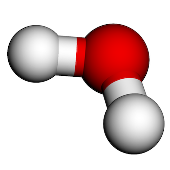
We’d like to derive an efficient algorithm that can take the number of electrons and the atomic numbers of the nuclei as input, and output an estimate for the bond lengths and angles. The algorithm should be broadly applicable and include as few assumptions as possible beyond the basic principles of quantum mechanics.

Note that efficiently simulating systems of point masses using classical Newtonian mechanics is relatively straightforward. For instance, consider a one-dimensional system of $N$ balls connected by springs. Each ball can be modeled by its position and each spring can be modeled by its length and stiffness.

We can use Hooke’s law to derive a system of $N$ quadratic equations relating the positions of the balls to the energy of the system. To solve for the state of the system at rest, we can minimize the energy by setting the derivative of the energy to zero and solving the resulting system of $N$ linear equations with $N$ variables. This method can be extended to arbitrary classical systems using the finite element method.

Extending this method to molecular simulation requires an efficient method for evaluating and minimizing the energy of a molecular state.

At the molecular level, the nuclei are heavy enough that it is common to approximate them as classical point masses that repel one-another according to Coulomb’s law. However, accurately simulating the electrons requires the application of quantum rather than classical mechanics.

The first difficulty this raises is that in quantum mechanics, the state of a particle can no longer be captured by position and velocity vectors. Rather, the state of a quantum particle is represented by a function over space called a wave function:

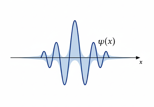
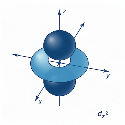
In particular, the state of an electron is represented by a three-dimensional wave function which in quantum chemistry is called an orbital. Each electron can occupy one of infinitely many orbitals. Here is a density plot of one of the hydrogen atom’s electron orbitals:

Efficiently encoding an electron orbital in computer memory already poses an interesting challenge. For example, one approach could be to discretize three dimensional space into cubes, and record the value of the wave function on each cube. Assuming a sparse discretization of just 100 points per dimension and using 32 bit floats for each cube, representing a single electron would require 4MB of memory. This is in contrast to 12 bytes to store the position vector of a classical particle.

This difference in the memory footprint is significant, but asymptotically it is merely a constant. A more significant challenge arises when considering how the state space scales with the number of electrons.

In classical mechanics, the state of $n$ particles is determined by a list of length $n$ containing the state of each particle. In contrast, the quantum state of $n$ particles is a superposition which is specified by assigning a probability amplitude to each possible length-$n$ list.

To be concrete, suppose for simplicity that both the classical and quantum particles may only be in one of two states: $0$ or $1$. The classical state of $n$ particles can be described by a length $n$ bit-string. On the other hand, the quantum state of $n$ particles is determined by assigning a probability amplitude to each possible length $n$ bit-string which requires $2^n$ complex numbers.

The fundamental challenge of quantum simulation is that the state space of $n$ particles grows exponentially with $n$.

In this series of posts we’ll introduce the Hartree-Fock method for approximating the ground state of a molecule.

To encode single-electron wave functions, the Hartree-Fock method fixes a finite basis set of wave functions (e.g Gaussians with different centers) and only considers wave functions in their span. Wave functions in this restricted set can be represented by their linear coefficients with respect to the basis.

To solve the exponential $n$-electron state space issue, Hartree-Fock only considers a small class of $n$-electron states called Slater determinants. The electronic ground state is then approximated by searching for the Slater determinant with the smallest expectation energy.

The algorithms in this series are implemented the slaterform library.

As an example, we can initialize a water molecule with the hydrogen atoms at an incorrect 180 degree angle, and then optimize its geometry by following the energy gradient. Here is a visualization of the resulting nuclei and electron density trajectories:

For more examples, see this colab notebook.

Nuclear State

The state of a nucleus is determined by its atomic number and its position.

Consider a molecule with $m$ nuclei. We’ll denote their atomic numbers by

\[Z = (Z_1,\dots,Z_m)\in\mathbb{Z}^m\]

and their positions by

\[\mathbf{R} = (\mathbf{R}_1,\dots,\mathbf{R}_m)\in\mathbb{R}^{3\times m}\]

The complete state of the nuclei, denoted $\mathcal{M}$, is specified by a tuple of atomic numbers $Z$ and positions $\mathbf{R}$:

\[\mathcal{M} = (\mathbf{R}, Z) \in \mathbb{R}^{3\times m} \times \mathbb{Z}^m\]

All quantities in this post are in atomic units.

Electronic State

In this section we’ll define the state space for a system of electrons.

Single Electron State

The state of a single electron has two components, one related to position in space and the other a quantum analog of angular momentum called spin.

The position is characterized by a wave function which is a complex valued square integrable function on $\mathbb{R}^3$:

\[\psi(\mathbf{r}) \in L^2(\mathbb{R}^3)\]

The space of square integrable complex valued functions on $\mathbb{R}^3$, $L^2(\mathbb{R}^3)$, is a Hilbert space where the inner product of two functions $\phi,\psi\in L^2(\mathbb{R}^3)$ is defined by:

\[\langle \phi | \psi \rangle := \int_{\mathbb{R}^3}\phi^*(\mathbf{r})\psi(\mathbf{r})d\mathbf{r}\]

The spin of an electron is a complex linear combination of two states called spin up and spin down. The spin component of the electron state can therefore be identified with the vector space $\mathbb{C}^2$.

Combining position and spin, the state space of an electron, denoted $\mathcal{H}$, is defined as the tensor product:

\[\mathcal{H} := L^2(\mathbb{R}^3)\otimes\mathbb{C}^2\]

The space $\mathcal{H}$ is also a Hilbert space since it’s a tensor product of two Hilbert spaces. Following standard quantum mechanics terminology, we’ll use the terms state space and Hilbert space interchangeably.

Anti-Symmetric tensors

To extend this to $n$ electrons, we’ll require the notion of an anti-symmetric tensor.

Following standard notation, we’ll denote the symmetric group of permutations of $n$ elements by $S_n$. We’ll also denote the sign of a permutation $\sigma\in S_n$ by $\mathrm{sgn}(\sigma)$

Definition (Symmetric Group Action). Let $V$ be a vector space and $n\in\mathbb{Z}$ a positive integer.

For each permutation $\sigma\in S_n$, define $P_\sigma\in\mathrm{Aut}(V^{\otimes n})$ to be the linear automorphism of $V^{\otimes n}$ defined on decomposable tensors by:

\[P_\sigma|v_1\dots v_N\rangle := |v_{\sigma^{-1}(1)}\dots v_{\sigma^{-1}(n)}\rangle\]

Definition (Anti-symmetric Tensor). Let $V$ be a vector space and $n\in\mathbb{Z}$ a positive integer.

A tensor $|v\rangle\in V^{\otimes n}$ is defined to be anti-symmetric if, for all $\sigma\in S_n$:

\[P_\sigma |v\rangle = \mathrm{sgn}(\sigma)|v\rangle\]

Since, for all $\sigma\in S_n$, $P_\sigma$ is a linear transformation of $V^{\otimes n}$, it follows that the set of anti-symmetric tensors is a subspace of $V^{\otimes n}$. This subspace is called the exterior product as formalized in the following definition.

Definition (Exterior Product). Let $V$ be a vector space and $n\in\mathbb{Z}$ a positive integer.

The $n$-th exterior product of $V$, denoted

\[\Lambda^n V \subset V^{\otimes n}\]

is defined to be the subspace of anti-symmetric tensors in $ V^{\otimes n}$.

According to the Pauli exclusion principle, the Hilbert space of a collection of $n$ electrons is equal to $\Lambda^n\mathcal{H}$. I.e, an $n$-electron state is an anti-symmetric tensor of $n$ single-electron states.

In quantum chemistry, elements of $\Lambda^n\mathcal{H}$ are referred to as molecular orbitals.

Slater Determinants

In the previous section we saw that the joint state space of $n$ electrons is equal to the exterior product $\Lambda^n\mathcal{H} \subset \mathcal{H}^{\otimes n}$.

Let $V$ be a vector space. The goal of this section is to show how to construct an anti-symmetric tensor in $\Lambda^n V$ from an arbitrary tensor $|v\rangle\in V^{\otimes n}$.

First we’ll consider the case where $n=2$. Consider the decomposable tensor:

\[|v_1 v_2\rangle \in V^{\otimes 2}\]

In general, $|v_1 v_2\rangle$ is not anti-symmetric. To see why, consider the permutation $\sigma=(1,2)\in S_2$. Then

\[P_\sigma |v_1 v_2\rangle = |v_2 v_1\rangle\]

Furthermore, $\mathrm{sgn}(\sigma) = -1$ and so

\[\mathrm{sgn}(\sigma)|v_1 v_2\rangle = -|v_1 v_2\rangle\]

Therefore, in general:

\[P_\sigma |v_1 v_2\rangle \neq \mathrm{sgn}(\sigma)|v_2 v_1\rangle\]

We can fix this by adding the missing term $-|v_2 v_1\rangle$ to our state and defining:

\[|v'\rangle = |v_1 v_2\rangle - |v_2 v_1\rangle\]

Now when we apply $P_\sigma$ we get:

\[\begin{align*} P_\sigma(|v'\rangle) &= P_\sigma |v_1 v_2\rangle - P_\sigma |v_2 v_1\rangle \\ &= |v_2 v_1\rangle - |v_1 v_2\rangle \\ &= -|v'\rangle \end{align*}\]

This implies that $|v’\rangle$ is an anti-symmetric tensor.

We can extend this construction to the case of $n$ electrons using the anti-symmetrization map $\mathcal{A}^n$ which maps the tensor product $V^{\otimes n}$ to the space of exterior product $\Lambda^n V$.

Definition (Anti-symmetrization). Let $V$ be a vector space and $n\in\mathbb{Z}$ a positive integer.

The anti-symmetrization map:

\[\mathrm{Alt}^n: V^{\otimes n} \rightarrow V^{\otimes n}\]

is defined by:

\[\mathrm{Alt}^n := \sum_{\sigma\in S_n}\mathrm{sgn}(\sigma) P_\sigma\]

Claim (Anti-symmetrization). Let $V$ be a vector space and $n\in\mathbb{Z}$ a positive integer.

Then, for all tensors $|v\rangle\in V^{\otimes n}$, $\mathrm{Alt}^n(|v\rangle)$ is an anti-symmetric tensor.

In particular, the image of the anti-symmetrization map is contained in $\Lambda^n V$:

\[\mathrm{Alt}^n : V^{\otimes n} \rightarrow \Lambda^n V\]

Proof [click to expand]

Let $|v\rangle\in V^{\otimes n}$ be a tensor. To show that $\mathrm{Alt}^n(|v\rangle)$ is anti-symmetric we must show that for all $\sigma\in S_n$,

\[P_\sigma \mathrm{Alt}^n(|v\rangle) = \mathrm{sgn}(\sigma)\mathrm{Alt}^n(|v\rangle).\]

Let $\sigma\in S_n$ be a permutation. Then, by the definition of the anti-symmetrization map:

\[\begin{align*} P_\sigma \mathrm{Alt}^n(|v\rangle) &= P_\sigma \sum_{\sigma'\in S_n}\mathrm{sgn}(\sigma') P_{\sigma'} |v\rangle \\ &= \sum_{\sigma'\in S_n}\mathrm{sgn}(\sigma)^2\mathrm{sgn}(\sigma') P_{\sigma\sigma'} |v\rangle \\ &= \mathrm{sgn}(\sigma)\sum_{\sigma'\in S_n}\mathrm{sgn}(\sigma\sigma') P_{\sigma\sigma'} |v\rangle \\ &= \mathrm{sgn}(\sigma) \mathrm{Alt}^n(|v\rangle) \end{align*}\]

The last equality follows from the fact that composition with $\sigma$ is an automorphism of $S_n$.

A convenient property of the anti-symmetrization map is that, up to a scalar, it is invariant to linear transformations of the input vectors:

Claim (Anti-Symmetrization Transformation). Let $V$ be a vector space, $n\in\mathbb{Z}$ a positive integer. $|v_1\rangle,\dots |v_n\rangle\in V$ vectors and $W\subset V$ their span:

\[W = \mathrm{Span}(|v_1\rangle,\dots,|v_n\rangle)\]

Let $T\in\mathrm{End}(W)$ be a linear transformation of $W$. Then:

\[\mathrm{Alt}^n(T|v_1\rangle \otimes\dots\otimes T|v_n\rangle) = \mathrm{det}(T)\mathrm{Alt}^n(|v_1\rangle \otimes\dots\otimes |v_n\rangle)\]

Proof [click to expand]

It’s easy to see that if the vectors $|v_1\rangle,\dots,|v_n\rangle$ are linearly dependent then $\mathrm{Alt}^n(|v_1\rangle\otimes\dots\otimes |v_n\rangle) = 0$. Therefore, we can assume that the vectors are linearly independent.

Since the vectors $|v_1\rangle,\dots,|v_n\rangle$ are linearly independent, $\mathrm{dim}W = n$ which implies that $\mathrm{dim}\Lambda^n W = 1$. Therefore, there exists a function

\[\lambda : \mathrm{End}(W) \rightarrow \mathbb{R}\]

such that for all $T\in\mathrm{End}(W)$:

\[\mathrm{Alt}^n(T|v_1\rangle\otimes\dots\otimes T|v_n\rangle) = \lambda(T) \mathrm{Alt}^n(|v_1\rangle\otimes\dots\otimes |v_n\rangle)\]

It remains to show that

\[\lambda(T) = \mathrm{det}(T)\]

where $\mathrm{det}(T)$ is the standard matrix determinant of $T$.

A transformation $T\in\mathrm{End}(W)$ is determined by its action on each of the basis vectors $|v_1\rangle,\dots,|v_n\rangle\in W$. In other words, there is an isomorphism

\[\mathrm{End}(W) \xrightarrow{\cong} W^n\]

which sends $T\in\mathrm{End}(W)$ to

\[(T\|v_1\rangle,\dots,T\|v_n\rangle)\in W^n\]

We can therefore realize the determinant as a function on $W^n$:

\[\mathrm{det}: W^n \rightarrow \mathbb{R}\]

This version of the determinant is characterized by the following three properties:

1. Normalized: It maps the basis $(|v_1\rangle,\dots,|v_n\rangle)$ to $1$.

2. Multi-linear: It is linear in each factor.

3. Alternating: If $(|w_1\rangle,\dots,|w_n\rangle)\in W^n$ and $w_i=w_j$ for some $i\neq j$ then $\mathrm{det}(w_1,\dots,w_n) = 0$.

It is easy to check that the function $\lambda$ defined above satisfies these properties.

q.e.d

In other words, transforming the input vectors has the effect of scaling their anti-symmetrization by the determinant of $T$.

The Slater determinant is a normalized version of the anti-symmetrization map.

Definition (Slater Determinant). Let $V$ be a vector space and $n\in\mathbb{Z}$ a positive integer.

The Slater determinant of the vectors $|v_1\rangle,\dots |v_n\rangle\in V$ is denoted by $|v_1,\dots,v_n\rangle$ (note the commas) and defined by:

\[|v_1,\dots,v_n\rangle := \frac{1}{\sqrt{n!}}\mathrm{Alt}^n(|v_1\dots v_n\rangle) \in \Lambda^n V\]

Closed Shell States

Recall that the Hilbert space $\mathcal{H}$ of single electron states is defined as:

\[\mathcal{H} := L^2(\mathbf{R}^3)\otimes \mathbb{C}^2\]

The seconds factor $\mathbb{C}^2$ represents the two-dimensional spin space spanned by spin down, denoted $|0\rangle$, and spin up, denoted $|1\rangle$.

Therefore, the decomposable single electron states $|\chi\rangle\in\mathcal{H}$ are of the form:

\[|\chi\rangle = |\psi\rangle |s\rangle\]

where $\psi\in L^2(\mathbf{R}^3)$ is a positional wave function and $s\in\{0,1\}$ indicates if the spin state is up or down.

In general, molecules are most stable when, for each positional wave function $|\psi\rangle$, either both or neither of the possible spin states are occupied. This type of electron configuration is called closed shell as formalized in the following definition.

Definition (Closed Shell Slater Determinant). Let $n\in\mathbb{Z}$ be an even integer and $\psi_1,\dots,\psi_{n/2}\in L^2(\mathbb{R}^3)$ positional wave functions.

The closed shell Slater determinant with positions $\psi_1,\dots,\psi_{n/2}$ is denoted $|\psi_1,\dots,\psi_n\rangle\in\Lambda^{n}(\mathcal{H})$ and defined to be the Slater determinant of the $n$ single-electron states

\[|\psi_1\rangle|0\rangle,|\psi_1\rangle|1\rangle,\dots, |\psi_n\rangle|0\rangle,|\psi_n\rangle|1\rangle \in \mathcal{H}\]

In other words, the closed shell Slater determinant of $\psi_1,\dots,\psi_{n/2}\in L^2(\mathbb{R}^3)$ is given by:

\[|\psi_1,\dots,\psi_n\rangle := |\psi_10,\psi_11,\dots,\psi_n0\psi_n1\rangle\in\Lambda^{n}(\mathcal{H})\]

Operators

In quantum mechanics, observables, including energy, correspond to self-adjoint operators of Hilbert space. We’ll be using the terms operator and linear transformation interchangeably.

In particular, the electronic energy of an $n$-electron molecule corresponds to a self-adjoint operator on $\Lambda^n\mathcal{H}$ called the Hamiltonian.

Let $V$ be a Hilbert space. In this section we’ll show how to construct self-adjoint operators on $\Lambda^n V$ from self-adjoint operators on $V^{\otimes k}$ for $1 \leq k \leq n$.

Symmetric Extension

Rather than directly constructing linear transformations of $\Lambda^n V$, we’ll instead construct linear transformations of $V^{\otimes n}$ that commute with the action of $S_n$ as formalized in the following definition.

Definition (Symmetric Operator). Let $V$ be a vector space and $n\in\mathbb{Z}$ a positive integer. An operator $T\in\mathrm{End}(V^{\otimes n})$ is defined to be symmetric if it commutes with the $S_n$ action on $V^{\otimes n}$.

In other words, $T$ is symmetric if for all $\sigma\in S_n$:

\[P_\sigma T = T P_\sigma\]

In our context, the significance of symmetric operators on $V^{\otimes n}$ is that they can be restricted to operators on $\Lambda^n V$.

Claim (Symmetric Restriction). Let $V$ be a vector space, $n\in\mathbb{Z}$ a positive integer and $T\in\mathrm{End}(V^{\otimes n})$ a symmetric operator on $V^{\otimes n}$.

Then, for any anti-symmetric tensor $|v\rangle\in V^{\otimes n}$, $T|v\rangle$ is also anti-symmetric. In particular, $T$ can be restricted to an operator on $\Lambda^n V$.

Proof [click to expand]

This follows immediately from the definition of an anti-symmetric tensor.

By Symmetric Restriction, in order to construct an operator on $\Lambda^n V$ it’s sufficient to construct a symmetric operator on $V^{\otimes n}$. We’ll now see how to build symmetric operators on $V^{\otimes n}$ from arbitrary operators on $V^{\otimes k}$ where $k \leq n$.

Definition (Symmetric Extension). Let $V$ be a vector space, $k \leq n\in\mathbb{Z}$ positive integers and $T^k\in\mathrm{End}(V^{\otimes k})$ an operator on $V^{\otimes k}$.

The symmetric extension of $T^k$, $T^n\in\mathrm{End}(V^{\otimes n})$, is defined to be:

\[T^n := \frac{1}{k!(n-k)!} \sum_{\sigma\in S_n} P_{\sigma^{-1}} (T^k \otimes \mathrm{Id}^{\otimes(n-k)}) P_{\sigma}\]

Claim (Symmetric Extension). Let $V$ be a vector space, $k \leq n\in\mathbb{Z}$ positive integers and $T^k\in\mathrm{End}(V^{\otimes k})$ an operator on $V^{\otimes k}$.

Then, the symmetrization extension of $T^k$, $T^n\in\mathrm{End}(V^{\otimes n})$, is a symmetric operator on $V^{\otimes n}$. In addition, if $T^k$ is self-adjoint then $T^n$ is self-adjoint.

Proof [click to expand]

First we’ll show that $T^n$ is symmetric. Let $\sigma\in S_n$ be a permutation.

Then, by the definition of $T^n$:

\[\begin{align*} P_{\sigma^{-1}} T^n P_{\sigma} &= P_{\sigma^{-1}} \left( \frac{1}{k!(n-k)!}\sum_{\sigma'\in S_n} P_{\sigma'^{-1}} (T^k \otimes \mathrm{Id}^{\otimes(n-k)}) P_{\sigma'}\right) P_{\sigma} \\ &= \frac{1}{k!(n-k)!}\sum_{\sigma'\in S_n} P_{(\sigma'\sigma)^{-1}} (T^k \otimes \mathrm{Id}^{\otimes(n-k)}) P_{\sigma'\sigma} \\ &= T^n \end{align*}\]

The last equality follows from the fact that $\sigma^{-1}$ is an automorphism of $S_n$.

Now suppose that $T^k$ is self adjoint, i.e, $(T^k)^* = T^k$. Note that $P_\sigma$ is unitary for all permutations $\sigma\in S_n$ which implies that:

\[\begin{align*} (T^n)^* &= (P_{\sigma^{-1}} (T^k \otimes \mathrm{Id}^{\otimes(n-k)}) P_\sigma)^* \\ &= P_\sigma^* (T^k \otimes \mathrm{Id}^{\otimes(n-k)}) P_{\sigma^{-1}}^* \\ &= P_{\sigma^{-1}} (T^k \otimes \mathrm{Id}^{\otimes(n-k)}) P_\sigma \\ &= T^n \end{align*}\]

This means that $T^n$ is a sum of self-adjoint operators which implies that it is self-adjoint.

The normalization constant of $\frac{1}{k!(n-k)!}$ was chosen so that, when $T^k$ is symmetric, its symmetric extension $T^n$ may be computed by applying $T^k$ to each size $k$ sub-factor of $V^{\otimes n}$ and taking the sum.

Before formalizing this result, let’s introduce some convenient notation for dealing with sequences of integers. For a given integer $n$, we’ll use the standard notation:

\[[n] := \{1,\dots,n\}\]

Given another integer $k$, we’ll denote the set of length $k$ sequences of integers in $[n]$ by $[n]^k$ and the set of length $k$ increasing sequences by $\binom{[n]}{k}\subset [n]^k$.

We can now state the formula alluded to above:

Claim (Symmetric Extension Formula). Let $V$ be a vector space, $k \leq n\in\mathbb{Z}$ positive integers, $T^k\in\mathrm{End}(V^{\otimes k})$ a symmetric operator and $T^n\in\mathrm{End}(V^{\otimes n})$ its symmetric extension.

For each increasing length $k$ sequence $I\in\binom{[n]}{k}$, let $T_I^n\in\mathrm{End}(V^{\otimes n})$ be the transformation that acts as $T^k$ on the factors of $V^{\otimes n}$ indexed by $I$ and as the identity to the remaining factors.

Then:

\[T^n = \sum_{I\in\binom{[n]}{k}} T_I^n\]

Proof [click to expand]

For a subsequence $I\in [n]^k$, we’ll use the notation $\mathrm{Im}(I)$ for the set of elements in $I$.

Now, note that if $I\in\binom{[n]}{k}$ is an increasing sequence and $\sigma\in S_n$ is a permutation satisfying

\[\mathrm{Im}(\sigma(I)) = [k]\]

then, since $T^k$ is symmetric:

\[T_I^n = P_{\sigma^{-1}}(T^k\otimes\mathrm{Id}^{n-k})P_\sigma\]

Recall that by definition:

\[T^n := \frac{1}{k!(n-k)!} \sum_{\sigma\in S_n} P_{\sigma^{-1}} (T^k \otimes \mathrm{Id}^{n-k}) P_{\sigma}\]

The claim now follows from the fact that, for each $I\in\binom{[n]}{k}$, there are $k!(n-k)!$ permutations $\sigma\in S_n$ satisfying:

\[\mathrm{Im}(\sigma(I)) = [k]\]

q.e.d

Expectation Value

An important notion in quantum mechanics is the expectation value of an operator in a given state:

Definition (Expectation Value). Let $V$ be a Hilbert space, let $|v\rangle\in V$ be a vector and $T\in\mathrm{End}(V)$ an operator.

The expectation value of $T$ in state $|v\rangle$ is defined to be:

\[\langle v | T | v \rangle\]

Let $V$ be a Hilbert space and $n\in\mathbb{Z}$ a positive integer.

Previously we’ve seen how to construct elements of $\Lambda^n V$ out of $n$ vectors $|v_1\rangle,\dots,|v_n\rangle\in V$ using a Slater determinant:

\[|v_1,\dots,v_n\rangle\in\Lambda^n V\]

In the previous section we saw how to use symmetric extension to construct an operator $T^n\in\mathrm{End}(\Lambda^n V)$ out of an operator $T^k\in\mathrm{End}(V^{\otimes k})$.

We’ll now derive a formula for the expectation value of $T^n$ in state $|v_1,\dots,v_n\rangle$ in terms of the operator $T^k$ and states $|v_1\rangle,\dots,|v_n\rangle$.

Given $n$ vectors $|v_1\rangle,\dots,|v_n\rangle\in V$ and a sequence $I = (i_1,\dots,i_k) \in [n]^k$ we’ll use the notation:

\[|v_I\rangle := |v_{i_1}\dots v_{i_k}\rangle \in V^{\otimes k}\]

Claim (Slater Determinant Expectation). Let $V$ be a Hilbert space and $k \leq n\in\mathbb{Z}$ positive integers.

Let $|v_1\rangle,\dots,|v_n\rangle\in V$ be orthonormal vectors in $V$. Let $T^k\in\mathrm{End}(V^{\otimes k})$ be a symmetric operator on $V^{\otimes k}$ and $T^n\in\mathrm{End}(V^{\otimes n})$ its symmetric extension.

Then:

\[\langle v_1,\dots,v_n | T^n | v_1,\dots,v_n \rangle = \frac{1}{k!}\sum_{ I\in [n]^k } \sum_{\sigma\in S_k} \mathrm{sgn}(\sigma) \langle v_I | T^k P_\sigma | v_I \rangle\]

Proof [click to expand]

To facilitation notation, we’ll define:

\[T_k^n := T^k\otimes\mathrm{Id}^{n-k}\]

By definition,

\[T^n = \frac{1}{k!(n-k)!}\sum_{ \rho \in S_n } P_{\rho^{-1}} T_k^n P_{\rho}\]

Also definition:

\[|v_1,\dots,v_n\rangle = \frac{1}{\sqrt{n!}} \sum_{\sigma \in S_n}\mathrm{sgn}(\sigma) P_{\sigma}|v_1 \dots v_n\rangle\]

Therefore,

\[\begin{align*} \langle v_1,\dots,v_n | T^n | v_1,\dots,v_n\rangle &= \frac{1}{k!(n-k)!n!} \sum_{\rho\in S_n} \sum_{\sigma,\sigma'\in S_n} \mathrm{sgn}(\sigma)\mathrm{sgn}(\sigma') \langle v_1\dots v_n | P_{\sigma^{-1}} P_{\rho^{-1}} T_k^n P_{\rho} P_{\sigma'} | v_1 \dots v_n \rangle \\ &= \frac{1}{k!(n-k)!n!} \sum_{\rho\in S_n} \sum_{\sigma,\sigma'\in S_n} \mathrm{sgn}(\sigma)\mathrm{sgn}(\sigma') \langle v_1\dots v_n | P_{(\rho\sigma)^{-1}} T_k^n P_{\rho\sigma'} | v_1 \dots v_n \rangle \\ &= \frac{1}{k!(n-k)!} \sum_{\sigma,\sigma'\in S_n} \mathrm{sgn}(\sigma)\mathrm{sgn}(\sigma') \langle v_1\dots v_n | P_{\sigma^{-1}} T_k^n P_{\sigma'} | v_1 \dots v_n \rangle \end{align*}\]

Now, let $\sigma,\sigma’\in S_n$ be permutations, and define the sequences $K :=(1,\dots,k)\in [n]^k$ and $K^c := (k+1,\dots,n)\in [n]^{n-k}$.

Since $T_k^n$ only acts on the first $k$ factors of $V^{\otimes n}$:

\[\langle v_1\dots v_n | P_{\sigma^{-1}} T_k^n P_{\sigma'} | v_1 \dots v_n \rangle = \langle v_{\sigma^{-1}(K)} | T^k | v_{\sigma'^{-1}(K)} \rangle \langle v_{\sigma^{-1}(K^c)} | v_{\sigma'^{-1}(K^c)} \rangle\]

By the orthonormality of $v_1,\dots,v_n$,

\[\langle v_{\sigma^{-1}(K^c)} | v_{\sigma'^{-1}(K^c)} \rangle = \begin{cases} 1 & \sigma'^{-1}(K^c) = \sigma^{-1}(K^c) \\ 0 & \mathrm{else} \end{cases}\]

We’ll now consider the non-zero case where $\sigma’^{-1}(K^c) = \sigma^{-1}(K^c)$.

First, note that in this case $\sigma^{-1}(K)$ and $\sigma’^{-1}(K)$ have the same elements. Therefore, there is a unique permutation $\tau\in S_k$ such that:

\[P_\tau |v_{\sigma^{-1}(K)}\rangle = |v_{\sigma'^{-1}(K)}\rangle\]

Note that since $\sigma’^{-1}(K) = \sigma^{-1}(K)$:

\[\mathrm{sgn}(\sigma)\mathrm{sgn}(\sigma') = \mathrm{sgn}(\tau)\]

Plugging this back into the above equation for the expectation value:

\[\begin{align*} \langle v_1,\dots,v_n | T^n | v_1,\dots,v_n\rangle &= \frac{1}{k!(n-k)!} \sum_{\sigma \in S_n} \sum_{\tau\in S_k} \mathrm{sgn}(\tau) \langle v_{\sigma^{-1}(K)} | T^k P_{\tau}| v_{\sigma^{-1}(K)} \rangle \\ \end{align*}\]

Let $P_{n,k}\subset [n]^k$ denote the set of sequences in $[n]^k$ that have unique elements. Note that $\sigma^{-1}(K)$ is in $P_{n,k}$ and that as $\sigma$ ranges over all permutations in $S_n$, each element of $P_{n,k}$ appears $(n-k)!$ times. Therefore, we can rewrite the sum as:

\[\begin{align*} \langle v_1,\dots,v_n | T^n | v_1,\dots,v_n\rangle &= \frac{1}{k!} \sum_{I \in P_{n,k}} \sum_{\tau\in S_k} \mathrm{sgn}(\tau) \langle v_{I} | T^k P_{\tau}| v_{I} \rangle \\ \end{align*}\]

To conclude the proof, we’ll show that the above sum can be replaced with a sum over all sequences in $[n]^k$ rather than just the ones with unique elements.

Let $I\in [n]^k$ be an arbitrary sequence. We claim that if the elements of $I$ are not unique then

\[\sum_{\tau\in S_k} \mathrm{sgn}(\tau) \langle v_I | T^k P_{\tau}| v_I \rangle = 0\]

To prove this, suppose that there exists $i\neq j \in [n]$ such that $I_i = I_j$ and let $(i,j)\in S_n$ denote the permutation that swaps $i$ and $j$.

Then

\[\begin{align*} \sum_{\tau\in S_k} \mathrm{sgn}(\tau) \langle v_I | T^k P_\tau| v_I \rangle &= \sum_{\tau\in S_k} \mathrm{sgn}(\tau(i,j) \langle v_I | T^k P_{\tau(i,j)}| v_I \rangle \\ &= -\sum_{\tau\in S_k} \mathrm{sgn}(\tau) \langle v_I | T^k P_\tau P_{(i,j)}| v_I \rangle \\ &= -\sum_{\tau\in S_k} \mathrm{sgn}(\tau) \langle v_I | T^k P_\tau| v_I \rangle \end{align*}\]

which implies that

\[\sum_{\tau\in S_k} \mathrm{sgn}(\tau) \langle v_I | T^k P_{\tau}| v_I \rangle = 0\]

q.e.d

An analogous formula holds for closed shell Slater determinants. The closed shell formula will make use of the number of cycles function

\[c : S_n \rightarrow \mathbb{Z}\]

which maps a permutation $\sigma\in S_n$ to the number of cycles in the cyclic decomposition of $\sigma$.

Claim (Closed Shell Expectation). Let $n\in\mathbb{Z}$ be an even integer, $T^k\in\mathrm{End}(L^2(\mathbb{R}^3)^{\otimes k})$ a symmetric operator and $T^n\in\mathrm{End}(\mathcal{H}^{\otimes n})$ the symmetric extension of $T^k\otimes\mathrm{Id}^{\otimes k} \in \mathrm{End}(\mathcal{H}^{\otimes k})$.

Let $|\psi_1\rangle,\dots,|\psi_{n/2}\rangle\in L^2(\mathbb{R}^3)$ be orthonormal positional wave functions.

Then:

\[\langle \psi_1,\dots,\psi_{n/2} | T^n | \psi_1,\dots,\psi_{n/2} \rangle = \frac{1}{k!} \sum_{I \in [n/2]^k}\sum_{\sigma\in S_k} 2^{c(\sigma)}\mathrm{sgn}(\sigma)\langle \psi_I | T^k P_{\sigma}| \psi_I \rangle\]

Proof [click to expand]

For each bit-string $s\in [2]^{n/2}$, we’ll define the spin state:

\[|s\rangle := |s_1\dots s_{n/2}\rangle \in \left(\mathbb{C}^2\right)^{\otimes (n/2)}\]

By Slater determinant expectation and the definition of $T^n$:

\[\langle \psi_1,\dots,\psi_{n/2} | T^{n} | \psi_1,\dots,\psi_{n/2} \rangle = \frac{1}{k!} \sum_{I\in [n/2]^k} \sum_{s \in [2]^k} \sum_{\sigma\in S_n} \langle \psi_I | T^k P_\sigma | \psi_I \rangle \langle s_I | P_\sigma | s_I \rangle\]

Let $t\in [2]^k$ be a bit-string and $\sigma\in S_k$ a permutation.

By the orthonormality of $|0\rangle,|1\rangle\in\mathbb{C}^2$:

\[\langle t | P_\sigma | t \rangle = \begin{cases} 1 & t = \sigma(t) \\ 0 & \mathrm{else} \end{cases}\]

If $\sigma$ is a cycle, then $t = \sigma(t)$ if and only if $t$ is all zeros or all ones. I.e, $t=(0,\dots,0)$ or $t=(1,\dots,1)$. This implies that for a general permutation $\sigma\in S_k$, the number of bit-strings $t\in [2]^k$ such that $t = \sigma(t)$ is equal to $2^{c(\sigma)}$.

Therefore:

\[\sum_{s \in [2]^k} \langle s_I | P_\sigma | s_I \rangle = 2^{c(\sigma)}\]

q.e.d

The following corollary is useful for computing the norm of a closed shell Slater determinant.

Claim (Closed Shell Norm). Let $n\in\mathbb{Z}$ be an even integer and $|\psi_1\rangle,\dots,\psi_{n/2}\rangle\in L^2(\mathbb{R}^3)$ orthonormal single-electron positional wave functions.

Then:

\[\langle \psi_1,\dots,\psi_{n/2} | \psi_1,\dots,\psi_{n/2} \rangle = \frac{2}{n}\sum_{i=1}^{n/2} \langle \psi_i | \psi_i \rangle\]

Proof [click to expand]

We’ll apply Closed Shell Expectation to the single-electron identity operator $T^1 = \mathrm{Id}\in\mathrm{End}(L^2(\mathbb{R}^3))$.

Let $T^{n}\in\mathrm{End}(\mathcal{H}^{\otimes n})$ be the symmetric extension of $T^1\otimes\mathrm{Id}\in\mathrm{End}(\mathcal{H})$.

By the definition of symmetric extension:

\[\begin{align*} T^n &= \frac{1}{(n - 1)!}\sum_{\sigma\in S_{n}}P_{\sigma^{-1}}T_1^1 P_\sigma \\ &= \frac{1}{(n - 1)!}\sum_{\sigma\in S_{n}}\mathrm{Id} \\ &= n\cdot\mathrm{Id} \end{align*}\]

Therefore:

\[\langle \psi_1,\dots,\psi_{n/2} | T^n | \psi_1,\dots,\psi_{n/2} \rangle = n \langle \psi_1,\dots,\psi_{n/2} | \psi_1,\dots,\psi_{n/2} \rangle\]

On the other hand, by Closed Shell Expectation:

\[\begin{align*} \langle \psi_1,\dots,\psi_{n/2} | T^n | \psi_1,\dots,\psi_{n/2} \rangle &= \sum_{i=1}^{n/2} 2^1 \langle \psi_i | T^1 | \psi_i \rangle \\ &= 2 \sum_{i=1}^{n/2} \langle \psi_i | \psi_i \rangle \end{align*}\]

The claim follows by combining the two equations above.

q.e.d

In particular, if the states $|\psi_1\rangle,\dots,\psi_{n/2}\rangle\in L^2(\mathbb{R}^3)$ are orthonormal then their closed shell Slater determinant has norm one.

The Electronic Hamiltonian

Our high level strategy for determining the ground state of a molecule is to search for the state with the smallest energy. The energy of a molecular state can be approximated as the sum of the energy of the nuclei and the energy of the electrons. Following the Born-Oppenheimer approximation, the energy of the nuclei is simply the sum of the classical Coulomb potential energy between each pair of electrons.

As we saw in Electronic State Space, the state of the electrons is a vector in $\Lambda^n\mathcal{H}$ where $n$ is the number of electrons. Therefore, the quantum energy of an electron state is determined by an operator on $\Lambda^n\mathcal{H}$. In quantum mechanics, the operator corresponding to the energy of a system is called the Hamiltonian.

The goal of this section is to rigorously define the Hamiltonian operator $H\in\mathrm{End}(\Lambda^n\mathcal{H})$ corresponding to the energy of a molecule’s electrons.

Since electrons have negative charge and nuclei have positive charge, the electronic energy can be expressed as a sum of the kinetic energies of the electrons, the potential energies of the electron-electron repulsions, and the potential energies of the electron-nuclei attractions.

We’ll start this section by defining self-adjoint operators on $\Lambda^n\mathcal{H}$ corresponding to each type of energy. The electronic Hamiltonian will then be defined to be their sum.

Kinetic Energy

The kinetic energy operator $T^1\in\mathrm{End}(L^2(\mathbb{R}^3))$ on the space of single-electron positional wave functions is defined by:

\[T^1 := -\frac{1}{2} \nabla^2 L^2(\mathbb{R}^3)\]

where $\nabla^2$ denotes the Laplace operator:

\[\nabla^2\psi = \frac{\partial^2}{\partial x^2}\psi + \frac{\partial^2}{\partial y^2}\psi + \frac{\partial^2}{\partial z^2}\psi\]

The Laplace operator is self-adjoint under the assumption that $\psi(\mathbf{r})$ goes to $0$ as $||\mathbf{r}||$ goes to infinity.

We can extend $T^1\in\mathrm{End}(L^2(\mathbb{R}^3))$ to an operator $T^1\otimes\mathrm{Id}\in\mathrm{End}(\mathcal{H})$ that acts trivially on the spin component.

The kinetic energy of $n$-electrons, denoted by $T^n\in\mathrm{End}(\Lambda^n\mathcal{H})$, is defined to be the symmetric extension of $T^1\otimes\mathrm{Id}$ from $\mathrm{End}(\mathcal{H})$ to $\mathrm{End}(\Lambda^n\mathcal{H})$.

Note that by Symmetric Extension Formula, applying $T^n$ to an $n$-electron state is equal to applying $T^1$ to the positional wave function of each electron and taking the sum. Similarly, the expected kinetic energy of a closed shell Slater determinant follows from Closed Shell Expectation:

Claim (Kinetic Energy Expectation). Let $n\in\mathbb{Z}$ be an even integer and $|\psi_1\rangle,\dots,|\psi_{n/2}\rangle\in L^2(\mathbb{R}^3)$ be orthonormal single-electron positional wave functions.

The expected kinetic energy of the closed shell Slater determinant $|\psi_1,\dots,\psi_{n/2}\rangle\in\Lambda^n \mathcal{H}$ is given by:

\[\langle \psi_1,\dots,\psi_{n/2} | T^n | \psi_1,\dots,\psi_{n/2} \rangle = 2\sum_{i=1}^{n/2} \langle \psi_i | T^1 | \psi_i \rangle\]

The inner products $\langle \psi_i | T^1 | \psi_i \rangle$ can be evaluated using the definition of $T^1$ and the definition of the inner product on $L^2(\mathbb{R}^3)$.

Claim (Kinetic Energy Integral). Let $\psi_1,\psi_2\in L^2(\mathbb{R}^3)$ be single-electron wave functions.

Then:

\[\langle \psi_1 | T^1 | \psi_2 \rangle = -\frac{1}{2} \int_{\mathbb{R}^3} \psi_1^*(\mathbf{r})\nabla^2\psi_2(\mathbf{r})d\mathbf{r}\]

Electron Nuclear Attraction

We’ll now consider the potential energy operator corresponding to the Coulomb attraction between electrons and nuclei.

Suppose that there are $m$ nuclei in state:

\[\mathcal{M} = (\mathbf{R}, Z) \in \mathbb{R}^{3\times m} \times \mathbb{Z}^m\]

The nuclear attraction operator for single-electron positional wave functions is an operator $V^1_{\mathrm{en}}(\mathbf{r};\mathcal{M})\in\mathrm{End}(L^2(\mathbb{R}^3))$ that acts as multiplication by

\[\phi_{\mathrm{en}}(\mathbf{r}; \mathcal{M}) := -\sum_{i=1}^m \frac{Z_i}{||\mathbf{R}_i - \mathbf{r}||} \in L^2(\mathbb{R}^3)\]

Specifically, given a positional wave function $\psi(\mathbf{r})\in L^2(\mathbb{R}^3)$:

\[V^1_{\mathrm{en}}(\mathbf{r}; \mathcal{M})\psi(\mathbf{r}) := \phi_{\mathrm{en}}(\mathbf{r}; \mathcal{M})\cdot\psi(\mathbf{r}) \in L^2(\mathbb{R}^3)\]

Since $V^1_{\mathrm{en}}(\mathbf{r};\mathcal{M})$ acts on the $L^2(\mathbb{R}^3)$ by multiplication by the real valued function $\phi_{\mathrm{en}}$, it is self-adjoint.

As usual, we can extend $V^1_{\mathrm{en}}(\mathbf{r}; \mathcal{M})\in\mathrm{End}(L^2(\mathbb{R}^3))$ to an operator $V^1_{\mathrm{en}}(\mathbf{r}; \mathcal{M})\otimes\mathrm{Id}\in\mathrm{End}(\mathcal{H})$ that acts trivially on the spin component.

The operator corresponding to the attraction between $n$ electrons and the $m$ nuclei, denoted by $V_{\mathrm{en}}^n(\mathbf{r}; \mathcal{M})\in\mathrm{End}(\Lambda^n\mathcal{H})$, is defined to be the symmetric extension of $V_{\mathrm{en}}^1(\mathbf{r}; \mathcal{M})\otimes\mathrm{Id}$ from $\mathrm{End}(\mathcal{H})$ to $\mathrm{End}(\Lambda^n\mathcal{H})$.

The nuclear attraction energy of a closed shell Slater determinant follows immediately from Closed Shell Expectation.

Claim (Nuclear Attraction Expectation). Let $m\in\mathbb{Z}$ be a positive integer and $\mathcal{M} \in \mathbb{R}^{3\times m} \times \mathbb{Z}^m$ a nuclear state.

Let $|\psi_1\rangle,\dots,|\psi_{n/2}\rangle\in L^2(\mathbb{R}^3)$ be orthonormal single-electron positional wave functions.

Then the expected nuclear attraction energy of the closed shell Slater determinant $|\psi_1,\dots,\psi_{n/2}\rangle\in\Lambda^n \mathcal{H}$ is given by:

\[\langle \psi_1,\dots,\psi_{n/2} | V^n_{\mathrm{en}}(\mathbf{r}; \mathcal{M}) | \psi_1,\dots,\psi_{n/2} \rangle = 2\sum_{i=1}^{n/2} \langle \psi_i | V^1_{\mathrm{en}}(\mathbf{r}; \mathcal{M}) | \psi_i \rangle\]

The single-electron inner-products can be evaluated using the definition of the inner product on $L^2(\mathbb{R}^3)$:

Claim (Nuclear Attraction Integral). Let $m\in\mathbb{Z}$ be a positive integer and

\[\mathcal{M} = (\mathbf{R}, Z) \in \mathbb{R}^{3\times m} \times \mathbb{Z}^m\]

a nuclear state.

Let $\psi_1,\psi_2\in L^2(\mathbb{R}^3)$ be single-electron wave functions.

Then:

\[\langle \psi_1 | V_{\mathrm{en}}^1(\mathbf{r}; \mathcal{M}) | \psi_2 \rangle = -\sum_{j=1}^m \int_{\mathbb{R}^3} \psi_1^*(\mathbf{r}) \frac{Z_j}{||\mathbf{R}_j - \mathbf{r}||}\psi_2(\mathbf{r}) d\mathbf{r}\]

Electron Repulsion

We’ll now consider the potential energy corresponding to the Coulomb repulsion between pairs of electrons.

First we’ll define Coulomb repulsion potential for a $2$-electron positional wave function as a symmetric operator $V_{\mathrm{ee}}^2\in\mathrm{End}(L^2(\mathbb{R}^3)^{\otimes 2}$.

For this purpose, we’ll use the canonical isomorphism between $L^2(\mathbb{R}^3) \otimes L^2(\mathbb{R}^3)$ and $L^2(\mathbb{R}^3\times\mathbb{R}^3)$:

\[\begin{align*} F: L^2(\mathbb{R}^3)\otimes L^2(\mathbb{R}^3) &\rightarrow L^2(\mathbb{R}^3\times\mathbb{R}^3) \\ (f(\mathbf{r}), g(\mathbf{r})) &\mapsto f(\mathbf{r}_1)\cdot g(\mathbf{r}_2) \end{align*}\]

The operator $V_{\mathrm{ee}}^2$ is defined on $L^2(\mathbb{R}^3\times\mathbb{R}^3)$ by multiplication by $\frac{1}{||\mathbf{r}_1 - \mathbf{r}_2||}$:

\[V_{\mathrm{ee}}^2\psi(\mathbf{r}_1,\mathbf{r}_2) := \frac{1}{||\mathbf{r}_1 - \mathbf{r}_2||} \cdot \psi(\mathbf{r}_1,\mathbf{r}_2)\]

Clearly $V_{\mathrm{ee}}^2$ commutes with the transposition of the coordinates $\mathbf{r}_1$ and $\mathbf{r}_2$. Therefore, under the canonical isomorphism $V_{\mathrm{ee}}^2$ is a symmetric operator on $L^2(\mathbb{R}^3)^{\otimes 2}$.

We can extend $V_{\mathrm{ee}}^2$ to a symmetric operator on $V_{\mathrm{ee}}^2\otimes\mathrm{Id}^{\otimes 2}\in\mathrm{End}(\mathcal{H}^{\otimes 2})$ that acts trivially on the spin factors $(\mathbb{C}^2)^{\otimes 2}$.

The Coulomb repulsion operator for $n$-electrons, denoted $V_{\mathrm{ee}}^n\in\mathrm{End}(\Lambda^n\mathcal{H})$, is defined as the symmetric extension of $V_{\mathrm{ee}}^2\otimes\mathrm{Id}^{\otimes 2}$ from $\mathrm{End}(\Lambda^2\mathcal{H})$ to $\mathrm{End}(\Lambda^n\mathcal{H})$.

Note that by Symmetric Extension Formula, applying $V_{\mathrm{ee}}^n$ to an $n$-electron state is equivalent to applying $V_{\mathrm{ee}}^2$ to each pair of electron positional wave-functions and taking the sum.

We can again apply Closed Shell Expectation to compute the expected election repulsion energy of a closed shell Slater determinant.

Claim (Electron Repulsion Expectation). Let $n\in\mathbb{Z}$ be an even integer. Let $|\psi_1\rangle,\dots,|\psi_{n/2}\rangle\in L^2(\mathbb{R}^3)$ be orthonormal single-electron positional wave functions.

The expected electron repulsion energy of the closed shell Slater determinant $|\psi_1,\dots,\psi_{n/2}\rangle\in\Lambda^n \mathcal{H}$ is given by:

\[\langle \psi_1,\dots,\psi_{n/2} | V_{\mathrm{ee}}^n | \psi_1,\dots,\psi_{n/2} \rangle = \sum_{i,j=1}^n \left( 2\langle \psi_i\psi_j | V_\mathrm{ee}^2 | \psi_i\psi_j \rangle - \langle \psi_i\psi_j | V_\mathrm{ee}^2 | \psi_j\psi_i \rangle \right)\]

Proof [click to expand]

By Closed Shell Expectation:

\[\begin{align*} \langle \psi_1,\dots,\psi_n | V_{\mathrm{ee}}^n | \psi_1,\dots,\psi_n \rangle &= \frac{1}{2}\sum_{i,j=1}^n \sum_{\sigma\in S_2} 2^{c(\sigma)}\mathrm{sgn}(\sigma) \langle \psi_i\psi_j |V_\mathrm{ee}^2 P_\sigma | \psi_i\psi_j \rangle \\ &= \sum_{i,j=1}^n\left( 2\langle \psi_i\psi_j | V_\mathrm{ee}^2 | \psi_i\psi_j \rangle - \langle \psi_i\psi_j | V_\mathrm{ee}^2 | \psi_j\psi_i \rangle\right) \end{align*}\]

q.e.d

The double-electron inner-products in the above claim can be computed as follows.

Claim (Electron Repulsion Integral). Let $n\in\mathbb{Z}$ be a positive integer and let $\psi_1,\dots,\psi_4\in L^2(\mathbb{R}^3)$ be single-electron wave functions.

Then:

\[\langle \psi_1\psi_2 | V_\mathrm{ee}^2 | \psi_3\psi_4 \rangle = \int_{\mathbb{R}^3}\int_{\mathbb{R}^3} \psi_1^*(\mathbf{r}_1)\psi_2^*(\mathbf{r}_2) \frac{1}{||\mathbf{r}_1 - \mathbf{r}_2||} \psi_3(\mathbf{r}_1)\psi_4(\mathbf{r}_2) d\mathbf{r}_1 d\mathbf{r}_2\]

Proof [click to expand]

The claim follows from the definition of $V_\mathrm{ee}^2$ and the definition of the inner-product on $L^2(\mathbb{R}^3\times\mathbb{R}^3)$.

q.e.d

The double-electron inner-products required by the SCF algorithm can be computed more efficiently by exploiting the following symmetry.

Claim (Electron Repulsion Symmetry). Let $n\in\mathbb{Z}$ be a positive integer and let $\psi_1,\dots,\psi_4\in L^2(\mathbb{R}^3, \mathbb{R})$ be real-valued single-electron wave functions.

Then the double-electron inner product is invariant to the following permutations:

\[\begin{align*} \langle \psi_1\psi_2 | V_\mathrm{ee}^2 | \psi_3\psi_4 \rangle &= \langle \psi_3\psi_2 | V_\mathrm{ee}^2 | \psi_1\psi_4 \rangle \\ &=\langle \psi_1\psi_4 | V_\mathrm{ee}^2 | \psi_3\psi_2 \rangle \\ &= \langle \psi_2\psi_1 | V_\mathrm{ee}^2 | \psi_4\psi_3 \rangle \end{align*}\]

This implies that to evaluate the double-electron inner product for all $24$ possible orderings of $\psi_1,\dots,\psi_4$, only $24/2^3 = 3$ of them must be computed.

The Hamiltonian

Consider a molecule with $m$ nuclei, $n$ electrons and nuclear state:

\[\mathcal{M} \in \mathbb{R}^{3\times m} \times \mathbb{Z}^m\]

The electronic Hamiltonian of the molecule, denoted $H^n(\mathbf{r};\mathcal{M}) \in \mathrm{End}(\Lambda^n\mathcal{H})$, is defined to be the sum of the kinetic, electron-nuclear and electron-electron operators defined above:

\[H^n(\mathbf{r};\mathcal{M}) := T^n + V_{\mathrm{en}}^n(\mathbf{r};\mathcal{M}) + V_{\mathrm{ee}}^n\]

The Schrodinger Equation

The time-independent Schrodinger equation determines the stationary states of a system with Hilbert space $V$ and Hamiltonian $H\in\mathrm{End}(V)$.

Specifically, it says that if $|v\rangle\in V$ is a stationary state with electronic energy $E\in\mathbb{R}$, then $|v\rangle$ is an eigenvector of $H$ with eigenvalue $E$:

\[H|v\rangle = E|v\rangle\]

In particular, the ground state of the system is given by the eigenvector of $H$ with the smallest eigenvalue.

In theory, all we need to do to determine the electronic ground state of a molecule with nuclear state $\mathcal{M}$ is to diagonalize the Hamiltonian $H^n(\cdot;\mathcal{M})\in\mathrm{End}(\Lambda^n\mathcal{H})$ and find the eigenvector with the smallest eigenvalue. In practice this is infeasible for all but the simplest systems.

To highlight the difficulty, note that the state space of $n$-electrons is equal to

\[\Lambda^n\mathcal{H} = \Lambda^n(L^2(\mathbb{R}^3)\otimes\mathbb{C}^2)\]

The set of integrable functions $L^2(\mathbb{R}^3)$ is infinite which means that we cannot directly express $H^n(\mathbf{r};\mathcal{M})\in\mathrm{End}(\Lambda^n\mathcal{H})$ as a matrix.

One idea could be to discretize $\mathbb{R}$ into a finite set of points and express a positional wave-function $\psi\in L^2(\mathbb{R}^3)$ in terms of the vector of its values on each point. However, even with a conservative discretization of only $100$ points per dimension, $L^2(\mathbb{R}^3)$ is $100^3$ dimensional and so $\Lambda^n(L^2(\mathbb{R}^3)\otimes\mathbb{C}^2)$ is $\binom{2 \cdot 100^3}{n}$ dimensional.

Rather than finding the exact ground state, we’ll instead use the Variational Principle to approximate it.

The Variational Principle

Consider a quantum system with Hilbert space $V$ and Hamiltonian $H\in\mathrm{End}(V)$. The Variational Principle states that for any state $|v\rangle\in V$ with norm $1$, the expectation energy of $|v\rangle$ is an upper bound on the ground state energy $E_0$:

\[\langle v | H | v \rangle \geq E_0\]

Furthermore, the inequality becomes exact when $|v\rangle$ is the ground state.

In our context, consider a molecule with nuclear state

\[\mathcal{M} \in \mathbb{R}^{3\times m} \times \mathbb{Z}^m\]

Let $H^n(\mathbf{r};\mathcal{M})\in\mathrm{End}(\Lambda^n\mathcal{H})$ be the electronic Hamiltonian of the molecule.

According to the variational principle, to find the electronic ground state we can search for an $n$-electron state $|\Psi\rangle\in\Lambda^n\mathcal{H}$ with unit norm that minimizes the expectation energy

\[\langle \Psi | H^n(\mathbf{r};\mathcal{M}) | \Psi \rangle\]

There are two major obstacles to this approach.

First, as mentioned in section The Schrodinger Equation, the space of $n$-electron states, $\Lambda^n\mathcal{H}$, is infinite dimensional.

The second issue is that evaluating inner products of the form $\langle \Psi | H^n(\mathbf{r};\mathcal{M}) | \Psi \rangle$ involves computing an integral over $\mathbb{R}^{3\times n}$ which is basically impossible to solve numerically.

Slater Determinant Optimization

As a first step to making the problem more tractable, we’ll restrict our search to $n$-electron states that are equal to the closed shell Slater determinant of $n/2$ orthonormal single-electron positional wave functions. In other words, we’ll try to minimize the energy of states $|\Psi\rangle$ of the form:

\[|\Psi\rangle = |\psi_1,\dots,\psi_{n/2}\rangle \in \Lambda^n\mathcal{H}\]

where $|\psi_1\rangle,\dots,|\psi_{n/2}\rangle\in L^2(\mathbb{R}^3)$ are orthonormal. Note that by Closed Shell Norm, $|\Psi\rangle$ has unit length.

More formally, we’ll introduce the Hartree-Fock energy functional which maps a list of positional wave functions to the expectation energy of their closed shell Slater determinant:

Definition (Hartree-Fock Energy Functional). Let $m\in\mathbb{Z}$ be a positive interger, $\mathcal{M}\in\mathbb{R}^{3\times m}\times\mathbb{Z}^m$ a nuclear state and $n\in\mathbb{Z}$ an even integer.

The Hartree-Fock energy functional is a function

\[E : L^2(\mathbb{R}^3)^{n/2} \rightarrow \mathbb{R}\]

defined by:

\[E(\psi_1,\dots,\psi_{n/2}; \mathcal{M}) := \langle\psi_1,\dots,\psi_{n/2} | H^n(\mathbf{r};\mathcal{M}) | \psi_1,\dots,\psi_{n/2}\rangle\]

We can restate our search for the electronic ground state as a constrained minimization of the Hartree-Fock functional. Specifically, our objective is to find single-electron wave functions $\psi_1,\dots,\psi_{n/2}\in L^2(\mathbb{R}^3)$ that minimize $E(\psi_1,\dots,\psi_{n/2}; \mathcal{M})$ subject to the orthonormality constraints:

\[\langle \psi_i | \psi_j \rangle = \delta_{ij}\]

for all $1 \leq i,j \leq n/2$ where $\delta_{ij}$ is the Kronecker delta.

The point of this reformulation is that we can solve this optimization problem using the method of Lagrange multipliers.

Following that method, we’ll introduce Lagrange multipliers $\lambda_{kl}\in\mathbb{R}$ where $1 \leq i,j \leq n/2$. We’ll then define the Lagrangian:

Definition (Hartree-Fock Lagrangian). Let $m\in\mathbb{Z}$ be a positive interger, $\mathcal{M}\in\mathbb{R}^{3\times m}\times\mathbb{Z}^m$ a nuclear state and $n\in\mathbb{Z}$ an even integer.

The Hartree-Fock Lagrangian is a function

\[L: L^2(\mathbb{R}^3)^{n/2} \times \mathbb{R}^{n/2 \times n/2} \rightarrow \mathbb{C}\]

defined by:

\[L(\psi_1,\dots,\psi_{n/2},\lambda_{0,0},\dots,\lambda_{n/2,n/2}; \mathcal{M}) := E(\psi_1,\dots,\psi_{n/2}; \mathcal{M}) - \sum_{i,j=0}^{n/2}\lambda_{ij}(\langle \psi_i | \psi_j \rangle - \delta_{kl})\]

By the theory of Lagrange multipliers, the minima of $E$ subject to the orthonormality constraints are critical points of $L$.

In order to formalize the notion of a critical point of $L$, we’ll start by defining a generalization of the derivative called the first variation.

Next we’ll introduce the Coulomb and exchange operators which are useful for concisely expressing the first variation of $L$.

Finally, we’ll put these two together and derive a necessary and sufficient condition for $(\psi_1,\dots,\psi_{n/2})\in L^2(\mathbb{R}^3)^{n/2}$ to be a critical point of $L$.

The First Variation

Let $f$ be a function defined on a product of Hilbert spaces. Intuitively, the first variation of $f$ is the best linear approximation to $f$. More formally:

Definition (First Variation). Let $n\in\mathbb{Z}$ be a positive integer, let $V_1,\dots,V_n$ be Hilbert spaces and $f:\prod_{i=1}^n V_i \rightarrow \mathbb{C}$ a function.

The first variation of $f$ at $(v_1,\dots,v_n)\in\prod_{i=1}^nV_i$ is a linear function

\[\delta f(v_1,\dots,v_n) : \prod_{i=1}^nV_i \rightarrow \mathbb{C}\]

that satisfies the property that for all $(\delta v_1,\dots,\delta v_n)\in\prod_{i=1}^nV_i$:

\[\begin{align*} f(v_1+\delta v_1,\dots,v_n+\delta v_n) &= f(v_1,\dots,v_n) + \delta f(v_1,\dots,v_n)[\delta v_1,\dots,\delta v_n] \\ &+ o(||(\delta v_1,\dots,\delta v_n)||) \end{align*}\]

In this definition we’re using the little-o notation for one function growing asymptotically faster than another one.

Here is a fundamental example of the first variation which is a generalization of the product rule for derivatives:

Claim (Matrix Element First Variation). Let $V$ be a Hilbert space, $A\in\mathrm{End}(V)$ an operator on $V$ and $f:V\times V\rightarrow\mathbb{C}$ the function defined by:

\[f(v,w) := \langle v | A | w \rangle\]

Then

\[\delta f(v,w)[\delta v,\delta w] = \langle \delta v | A | w \rangle + \langle v | A | \delta w \rangle\]

Proof [click to expand]

The proof follows by direct calculation:

\[\begin{align*} \langle v + \delta v | A | w +\delta w \rangle &= \langle v | A | w \rangle + \langle \delta v | A | w \rangle + \langle v | A | \delta w \rangle + \langle \delta v | A | \delta w \rangle \\ &= \langle v | A | w \rangle + (\langle \delta v | A | w \rangle + \langle v | A | \delta w \rangle) + o(||(\delta v, \delta w)||) \end{align*}\]

When the arguments of $\delta f$ are clear from the context, we will omit them. For example, we’ll sometimes write the statement of the previous claim as:

\[\delta \langle v | A | w \rangle = \langle \delta v | A | w \rangle + \langle v | A | \delta w \rangle\]

The following special case will be useful as well.

Claim (Expectation First Variation). Let $V$ be a Hilbert space, $A\in\mathrm{End}(V)$ a self-adjoint operator on $V$ and $f:V\times V\rightarrow\mathbb{C}$ the function defined by:

\[f(v) := \langle v | A | v \rangle\]

Then

\[\delta f = 2\mathrm{Re}(\langle \delta v | A | v \rangle)\]

Proof [click to expand]

Consider the function $B: V \times V \rightarrow \mathbb{C}$ defined by:

\[B(v_1,v_2) := \langle v_1 | A | v_2 \rangle\]

By Matrix Element First Variation, the first variation of $B$ is given by:

\[\delta B = \langle\delta v_1 | A | v_2 \rangle + \langle v_1 | A | \delta v_2 \rangle\]

Let $g:V \rightarrow V\times V$ denote the diagonal map defined by $g(v) = (v,v)$. Applying the chain rule to $B\circ g$:

\[\begin{align*} \delta\langle v | A | v \rangle &= \langle \delta v | A | v \rangle + \langle v | A | \delta v \rangle \\ &= \langle \delta v | A | v \rangle + \langle \delta v | A | v \rangle^* \\ &= 2\mathrm{Re}(\langle \delta v | A | v \rangle) \end{align*}\]

q.e.d

Trace And Density

The most complicated part of the electronic Hamiltonian $H^n(\mathbf{r};\mathcal{M})$ is the Coulomb repulsion potential between each pair of electrons.

Interestingly, as we will see in the following sections, the solutions to the constrained Hartree-Fock energy functional minimization can be expressed in terms of the Coulomb repulsion between each electron and the average over the other electrons.

This has the effect of replacing a quadratic expression with a linear one and is the primary computation advantage of restricting our search to closed shell Slater determinants.

In this section we’ll introduce the notion of the trace of an operator which formalizes the notion of averaging the value of an operator over space. We’ll then define the density operator which is a way of representing a collection of quantum states. In the next section we’ll define the Coulomb and exchange operators as the trace the Coulomb potential with respect to a given density.

The trace of a matrix is defined as the sum of the diagonal elements. Similarly, the trace of a linear operator over Hilbert space is defined as the sum over the diagonal matrix elements.

Definition (Trace). Let $V$ be a Hilbert space and $|i\rangle$ for $i\in\mathbb{Z}$ be an orthonormal basis of $V$.

The trace is a linear map:

\[\mathrm{Tr}: \mathrm{End}(V)\rightarrow\mathbb{C}\]

defined on an operator $A\in\mathrm{End}(V)$ by:

\[\mathrm{Tr}(A) := \sum_i \langle i | A | i \rangle\]

It is possible to show that the trace is independent of the chosen basis $|i\rangle$.

Intuitively, we can think of the trace as integrating the kernel $A$ over $V$.

When the underlying space is a tensor product $V\otimes W$, we can take the trace with respect to just one of the factors by summing over that factors basis.

Definition (Partial Trace). Let $V$ and $W$ be Hilbert spaces and $|i\rangle$ for $i\in\mathbb{Z}$ an orthonormal basis of $W$.

The partial trace over $W$ is a linear map

\[\mathrm{Tr}_W: \mathrm{End}(V\otimes W) \rightarrow \mathrm{End}(V)\]

defined on an operator $A\in\mathrm{End}(V\otimes W)$ by:

\[\mathrm{Tr}_W(A) := \sum_i (\mathrm{Id}_V \otimes \langle i |) A (\mathrm{Id}_V \otimes |i \rangle)\]

Similarly to the trace, this definition is independent of the orthonormal basis on $W$. When $V=W$, we’ll denote the partial trace on $\mathrm{End}(V\otimes V)$ with respect to the second factor by $\mathrm{Tr}_2$.

Intuitively, the partial trace can be thought of as integrating out the kernel $A$ over $W$ to obtain a kernel on $V$ only.

We’ll now show how the trace can be used to compactly represent the expectation value of a collection of states.

Claim (Expectation From Trace). Let $V$ be a Hilbert space, $A$ an operator on $V$ and $|v\rangle\in V$ a vector.

Then:

\[\langle v | A | v \rangle = \mathrm{Tr}(|v\rangle\langle v| A)\]

Proof [click to expand]

Let $|i\rangle$ be an orthonormal basis of $V$. Then:

\[\begin{align*} \mathrm{Tr}(|v\rangle\langle v| A) &= \sum_{i=1}\langle i | v \rangle \langle v | A | i \rangle \\ &= \langle v | A | \sum_{i=1}\langle i | v \rangle i \rangle \\ &= \langle v | A | v \rangle \end{align*}\]

q.e.d

Now consider a collection of states $|v_1\rangle,\dots,|v_n\rangle\in V$. By linearity of the trace, the sum of the expectations is:

\[\begin{equation}\label{eq:expectation-trace} \sum_i \langle v_i | A | v_i \rangle = \mathrm{Tr}\left(\sum_i |v_i\rangle\langle v_i | A\right) \end{equation}\]

This motivates the following definition:

Definition (Density Operator). Let $V$ be a Hilbert space, $n\in\mathbb{Z}$ an integer and $|v_1\rangle,\dots,|v_n\rangle\in V$ orthonormal vectors.

The corresponding density operator, $\rho\in\mathrm{End}(V)$ is defined to be:

\[\rho := \sum_{i=1}^n |v_i\rangle\langle v_i|\]

We can now rewrite the above equation \ref{eq:expectation-trace} using the density operator:

Claim (Trace of a Density Operator). Let $V$ be a Hilbert space, $n\in\mathbb{Z}$ an integer, $A\in\mathrm{End}(V)$ an operator on $V$, $|v_1\rangle,\dots,|v_n\rangle\in V$ orthonormal vectors and $\rho\in\mathrm{End}(V)$ the corresponding density operator

Then

\[\sum_{i=1}^n \langle v_i | A | v_i \rangle = \mathrm{Tr}(\rho A)\]

This is analogous to the definition of the expected value as a weighted average.

We can also use the partial trace to integrate over one factor of a tensor product $V\otimes W$ with respect to a density operator on that factor:

Claim (Partial Trace of a Density Operator). Let $V$ and $W$ be Hilbert spaces, $n\in\mathbb{Z}$ be an integer, $A\in\mathrm{End}(V\otimes W)$ an operator on $V\otimes W$, $|w_1\rangle,\dots,|w_n\rangle\in W$ orthonormal vectors and $\rho_W\in\mathrm{End}(W)$ the corresponding density operator.

Then

\[\sum_i (\mathrm{Id}_V\otimes \langle w_i|) A (\mathrm{Id}_V\otimes | w_i \rangle) = \mathrm{Tr}_W(\rho A)\]

One useful property of density operators is that they are invariant to unitary transformations of the constituent vectors:

Claim (Density Operator Invariance). Let $V$ be a Hilbert space, $n\in\mathbb{Z}$ an integer, $|v_1\rangle,\dots,|v_n\rangle\in V$ orthonormal vectors and $\rho\in\mathrm{End}(V)$ the associated density operator.

Let $U\in\mathrm{End}(V)$ be a unitary transformation that maps the span of the $|v_i\rangle$ to itself.

Then, the density operator corresponding to the transformed vectors $U|v_1\rangle,\dots,U|v_n\rangle$ is also equal to $\rho$.

Proof [click to expand]

Let $\rho_U$ denote the density operator corresponding to $U|v_1\rangle,\dots,U|v_n\rangle$. By definition:

\[\begin{align*} \rho_U &= \sum_{i=1}^n U|v_i\rangle\langle v_i|U^* \\ &= U \rho U^* \end{align*}\]

Now note that $\rho$ is the projection operator onto

\[W := \mathrm{Span}(|v_1\rangle,\dots,|v_n\rangle)\]

Since by assumption $U$ maps $W$ to itself, $U \rho U^*$ is also the projection onto $W$.

q.e.d

Finally, it will also be useful to define the closed shell analog of the density operator.

Definition (Closed Shell Density Operator). Let $n\in\mathbb{Z}$ be an even integer and $|\psi_1\rangle,\dots,|\psi_{n/2}\rangle\in L^2(\mathbb{R}^3)$ orthonormal positional wave-functions.

The associated closed-shell density operator, $\rho\in\mathrm{End}(L^2(\mathbb{R}^3))$ is defined by:

\[\rho := 2 \sum_{i=1}^{n/2}|\psi_i\rangle\langle\psi|\]

The factor of $2$ accounts for the fact that, in a closed shell state, each positional wave-function $|\psi_i\rangle$ represents two electrons: one with spin up and one with spin down.

Coulomb And Exchange Operators

In section Electron Repulsion we defined the electron-electron repulsion operator $V_\mathrm{ee}\in\mathrm{End}(L^2(\mathbb{R}^3)^{\otimes 2})$ between a pair of electrons. Intuitively, the Coulomb operator represents the average repulsion between a single electron and an electron density distribution.

Definition (Coulomb Operator). Let $\rho\in\mathrm{End}(L^2(\mathbb{R}^3))$ be a density operator.

The Coulomb operator associated to $\rho$ is an operator $J(\rho)\in\mathrm{End}(L^2(\mathbb{R}^3))$ defined by:

\[J(\rho) := \mathrm{Tr}_2 \left( (\mathrm{Id} \otimes \rho) V_\mathrm{ee}^2 \right)\]

The exchange operator is defined similarly by composing the electron-electron repulsion operator with the permutation operator

\[P_{(1,2)}\in\mathrm{End}(L^2(\mathbb{R}^3)^{\otimes 2})\]

that exchanges the two electrons.

Definition (Exchange Operator). Let $\rho\in\mathrm{End}(L^2(\mathbb{R}^3))$ be a density operator.

The exchange operator associated to $\rho$ is an operator on $K(\rho)\in\mathrm{End}(L^2(\mathbb{R}^3))$ defined by:

\[K(\rho) := \mathrm{Tr}_2 \left( (\mathrm{Id} \otimes \rho) V_\mathrm{ee}^2 P_{(1,2)} \right)\]

The Fock Operator

We are now ready to characterize the solutions to the constrained minimization of the Hartree-Fock energy functional $E$.

By the method of Lagrange multipliers, solutions to the constrained minimization of $E$ are critical points of the Hartree-Fock Lagrangian $L$.

In other words, if $(\psi_1,\dots,\psi_{n/2})\in L^2(\mathbb{R}^3)^{n/2}$ is a solution to the constrained optimization problem, then there exist Lagrange multipliers $\lambda_{ij}\in\mathbb{R}$ such that:

\[\delta L(\psi_1,\dots,\psi_{n/2},\lambda_{0,0},\dots,\lambda_{n/2,n/2};\mathcal{M}) = 0\]

By the definition of $L$ and linearity of the first variation, this implies that the solution satisfies:

\[\begin{equation}\label{eq:energy-variation} \delta E(\psi_1,\dots,\psi_n; \mathcal{M}) = \sum_{i,j=1}^{n/2}\lambda_{ij} \delta \langle \psi_i | \psi_j \rangle \end{equation}\]

We can use Closed Shell Expectation to compute the left hand side of equation \ref{eq:energy-variation} in terms of single and double electron operators. To facilitate notation, we’ll define the single-electron Hamiltonian

\[H^1(\mathbf{r};\mathcal{M}) \in \mathrm{End}(L^2(\mathbb{R}^3))\]

as the sum of the single-electron kinetic energy and electron-nuclear attraction operators:

\[H^1(\mathbf{r}; \mathcal{M}) := T^1 + V^1_{\mathrm{en}}(\mathbf{r};\mathcal{M})\]

Claim (Hartree-Fock Energy Variation). Let $m\in\mathbb{Z}$ be a positive integer and $\mathcal{M}\in\mathbb{R}^{3\times m}\times\mathbb{Z}^m$ a nuclear state.

Let $n\in\mathbb{Z}$ be an even integer, $|\psi_1\rangle,\dots,|\psi_{n/2}\rangle\in L^2(\mathbb{R}^3)$ orthonormal single-electron states and $\rho\in\mathrm{End}(L^2(\mathbb{R}^3))$ the corresponding closed shell density operator.

Then

\[\delta E(\psi_1,\dots,\psi_{n/2}; \mathcal{M}) = 4\mathrm{Re}\left( \sum_{i=1}^{n/2}\langle \delta\psi_i | H^1(\mathbf{r};\mathcal{M}) + J(\rho) - \frac{1}{2}K(\rho) | \psi_i\rangle \right)\]

Proof [click to expand]

By definition,

\[H^n(\mathbf{r};\mathcal{M}) = T^n + V_\mathrm{en}^n(\mathbf{r};\mathcal{M}) + V_\mathrm{ee}^n\]

Recall from section The Electronic Hamiltonian that $T^n$ and $V_\mathrm{en}^n(\mathbf{r};\mathcal{M})$ are defined to be the symmetric extensions of the single-electron operators $T^1\in\mathrm{End}(L^2(\mathbb{R}^3))$ and $V_\mathrm{en}^1(\mathbf{r};\mathcal{M})\in\mathrm{End}(L^2(\mathbb{R}^3))$.

Similarly, $V_\mathrm{ee}^n$ is defined to be the symmetric extension of the double electron operator $V_\mathrm{ee}^2\in\mathrm{End}(L^2(\mathbb{R}^3)^{\otimes 2})$.

We’ll split the functional $E$ into two components by defining

\[E_1(\psi_1,\dots,\psi_{n/2}) := \langle \psi_1,\dots,\psi_{n/2} | T^n + V_\mathrm{en}^n(\mathbf{r};\mathcal{M}) | \psi_1,\dots,\psi_{n/2} \rangle\]

and

\[E_2(\psi_1,\dots,\psi_{n/2}) := \langle \psi_1,\dots,\psi_{n/2} | V_\mathrm{ee}^n | \psi_1,\dots,\psi_{n/2} \rangle\]

We’ll start by evaluating $\delta E_1$.

By Closed Shell Expectation:

\[E_1(\psi_1,\dots,\psi_{n/2}) = 2\sum_{j=1}^{n/2}\langle \psi_j | H^1(\mathbf{r};\mathcal{M}) | \psi_j \rangle\]

Therefore, by Expectation First Variation:

\[\delta E_1 = 4\mathrm{Re}\left( \sum_{j=1}^{n/2}\langle \delta\psi_i | H^1(\mathbf{r};\mathcal{M}) | \psi_i \rangle \right)\]

The analysis for $E_2$ is similar. To facilitate notation, we’ll define:

\[H^2 := V_\mathrm{ee}^2(\mathrm{Id} - \frac{1}{2}P_{(1,2)})\]

By Electron Repulsion Expectation:

\[E_2(\psi_1,\dots,\psi_{n/2}) = 2\sum_{i,j=1}^{n/2} \langle\psi_i\psi_j | H^2 | \psi_i\psi_j\rangle\]

Similarly to Expectation First Variation, it’s easy to see that:

\[\delta \langle\psi_i\psi_j | H^2 | \psi_i\psi_j\rangle = 2\mathrm{Re}( \langle\delta\psi_i\psi_j | H^2 | \psi_i\psi_j\rangle +\langle\psi_i\delta\psi_j | H^2 | \psi_i\psi_j\rangle)\]

Furthermore, note that:

\[\langle\psi_i\delta\psi_j | H^2 | \psi_i\psi_j\rangle = \langle\delta\psi_j\psi_i | H^2 | \psi_j\psi_i\rangle\]

Together we obtain:

\[\delta E_2 = 4\mathrm{Re}\left( 2\sum_{i,j=1}^{n/2} \langle\delta\psi_i\psi_j | H^2 | \psi_i\psi_j\rangle \right)\]

Finally, by Partial Trace of a Density Operator it follows that for all $1\leq i \leq n/2$:

\[\begin{align*} 2\sum_{j=1}^{n/2} \langle\delta\psi_i\psi_j | H^2 | \psi_i\psi_j\rangle &= 2\langle \delta\psi_i | \sum_{j=1}^{n/2}( (\mathrm{Id}\otimes\langle\psi_j |) H^2 (\mathrm{Id}\otimes | \psi_j\rangle) |\psi_i\rangle \\ &= \langle \delta\psi_i | \mathrm{Tr}_2 (\rho H^2) | \psi_i \rangle \\ &= \langle \delta\psi_i | J(\rho) - \frac{1}{2}K(\rho) | \psi_i \rangle \end{align*}\]

q.e.d

This motivates the definition of the Fock operator

Definition (Fock Operator). Let $m\in\mathbb{Z}$ be a positive integer, $\mathcal{M}\in\mathbb{R}^{3\times m}\times\mathbb{Z}^m$ a nuclear state and $\rho\in\mathrm{End}(L^2(\mathbb{R}^3))$ a density operator.

The Fock operator associated to the molecule $\mathcal{M}$ and electron density $\rho$ is an operator $F(\mathbf{r}; \rho,\mathcal{M})\in\mathrm{End}(L^2(\mathbb{R}^3))$ defined by:

\[F(\mathbf{r}; \rho,\mathcal{M}) := H^1(\mathbf{r};\mathcal{M}) + J(\rho) - \frac{1}{2}K(\rho)\]

Returning to equation \ref{eq:energy-variation}, by Matrix Element First Variation, the first variation of the right-hand side is given by:

\[\sum_{i,j=1}^{n/2}\lambda_{ij} \delta \langle \psi_i | \psi_j \rangle = 2\mathrm{Re}\left(\sum_{i,j=1}^{n/2} \lambda_{ij}\langle \delta\psi_i | \psi_j\rangle\right)\]

Substituting this equality and Hartree-Fock Energy Variation back into equation \ref{eq:energy-variation}:

\[4\mathrm{Re}\left( \sum_{i=1}^{n/2}\langle \delta\psi_i | F(\rho, \mathbf{R}, Z) | \psi_i\rangle \right) = 2\mathrm{Re}\left(\sum_{i,j=1}^{n/2} \lambda_{ij}\langle \delta\psi_i | \psi_j \rangle\right)\]

Since this holds for all $|\delta\psi_i\rangle\in L^2(\mathbb{R}^3)$, it follows that for all $1\leq i \leq n/2$:

\[\begin{equation}\label{eq:fock-invariant-subspace} F(\mathbf{r}; \rho,\mathcal{M}) | \psi_i\rangle = \frac{1}{2}\sum_{j=1}^{n/2} \lambda_{ij} |\psi_j\rangle \end{equation}\]

Let $V\subset L^2(\mathbb{R}^3)$ be the span of $|\psi_1\rangle,\dots,|\psi_{n/2}\rangle$:

\[V := \mathrm{Span}(|\psi_1\rangle,\dots,|\psi_{n/2}\rangle)\]

Equation \ref{eq:fock-invariant-subspace} is equivalent to the condition that the operator $F(\mathbf{r}; \rho,\mathcal{M})$ maps $V$ to itself.

We can summarize the above discussion as follows:

Claim (Hartree-Fock Local Minima). Let $m\in\mathbb{Z}$ be a positive integer and $\mathcal{M}\in\mathbb{R}^{3\times m}\times\mathbb{Z}^m$ a nuclear state.

Let $n\in\mathbb{Z}$ be an even integer, $|\psi_1\rangle,\dots,|\psi_{n/2}\rangle \in L^2(\mathbb{R}^3)$ orthonormal wave-functions, $V\subset L^2(\mathbb{R}^3)$ their span and $\rho\in\mathrm{End}(L^2(\mathbb{R}^3))$ the associated closed-shell density operator.

Then, the states $|\psi_1\rangle,\dots,|\psi_{n/2}\rangle$ are a local minimum of the Hartree-Fock energy functional $E(\cdot ; \mathcal{M})$ with respect to the orthonormality constraint iff:

\[F(\mathbf{r}; \rho, \mathcal{M})V \subset V\]

W can simplify further by noting that by Anti-Symmetrization Transformation, if $U\in\mathrm{End}(V)$ is a unitary transformation then

\[|U\psi_1,\dots,U\psi_{n/2}\rangle = \mathrm{det}(U)|\psi_1,\dots,\psi_{n/2}\rangle\]

In other words, the electron state $|\psi_1,\dots,\psi_{n/2}\rangle$ is, up to a phase, invariant to unitary transformations of $V$. This means that we are free to replace the local minimum $|\psi_1\rangle,\dots,|\psi_{n/2}\rangle$ with any orthonormal basis of $V$ without affecting the resulting ground state.

Since $F(\mathbf{r}; \rho,\mathcal{M})$ is Hermitian, a natural candidate for such a basis is an orthonormal basis of eigenvectors of $F(\mathbf{r}; \rho,\mathcal{M})$. Let $|\psi’_1\rangle,\dots,|\psi’_{n/2}\rangle$ be an orthonormal eigenbasis and $\lambda’_1,\dots,\lambda’_{n/2}\in\mathbb{R}$ the corresponding eigenvalues. By definition, for all $1\leq i \leq n/2$:

\[F(\mathbf{r}; \rho, \mathcal{M}) |\psi'_i\rangle = \lambda'_i |\psi'_i\rangle\]

Furthermore, by Density Operator Invariance, the density operator $\rho’\in\mathrm{End}(L^2(\mathbb{R}))$ corresponding to the eigenvectors $|\psi’_i\rangle$ is equal to the original density $\rho$. Therefore:

\[F(\mathbf{r}; \rho', \mathcal{M}) |\psi'_i\rangle = \lambda'_i |\psi'_i\rangle\]

This motivates the introduction of the Fock equation.

Definition (Fock Equation). Let $m\in\mathbb{Z}$ be a positive integer and $\mathcal{M}\in\mathbb{R}^{3\times m}\times\mathbb{Z}^m$ a nuclear state.

Let $n\in\mathbb{Z}$ be an even integer, $|\psi_1\rangle,\dots,|\psi_{n/2}\rangle \in L^2(\mathbb{R}^3)$ orthonormal wave-functions and $\rho\in\mathrm{End}(L^2(\mathbb{R}^3))$ the associated closed-shell density operator.

The Fock equation states that:

\[F(\mathbf{r}; \rho, \mathcal{M}) |\psi_i\rangle = \lambda_i |\psi_i\rangle\]

for some eigenvalues $\lambda_1,\dots,\lambda_{n/2}\in\mathbb{R}$.

By Hartree-Fock Local Minima, any solution to the Fock equation is a local minimum of the Hartree-Fock energy functional subject to the orthonormality constraint. Conversely, by the discussion above, any local minimum can be transformed to a solution to the Fock equation without affecting the associated electron state.

Note that in the Fock equation the density operator $\rho$ depends on the the states $|\psi_i\rangle$. Therefore, we cannot simply solve for eigenvectors of $F(\mathbf{r}; \rho, \mathcal{M})$. We’ll instead apply an iterative approach which alternates between fixing $\rho$ and solving for the eigenvectors of $F(\mathbf{r}; \rho, \mathcal{M})$, and between constructing a new density $\rho$ from the current eigenvectors.

One obstacle to this plan is that the space $L^2(\mathbb{R}^3)$ of single electron positional states is infinite dimensional. The goal of the next section is to apply this theory to a finite dimensional approximation.

We’ll conclude this section by noting that the Hartree-Fock energy functional can be expressed in terms of the Fock operator. The utility of this is that, after the iterative process outlined above converges, we can reuse the resulting Fock operator to compute the expectation energy at the converged point.

Claim (Expectation Energy From Fock). Let $m\in\mathbb{Z}$ be a positive integer and $\mathcal{M}\in\mathbb{R}^{3\times m}\times\mathbb{Z}^m$ a nuclear state.

Let $n\in\mathbb{Z}$ be an even integer, $|\psi_1\rangle,\dots,|\psi_{n/2}\rangle \in L^2(\mathbb{R}^3)$ orthonormal states and $\rho\in\mathrm{End}(L^2(\mathbb{R}^3))$ the associated closed shell density operator. Then:

\[E(\psi_1,\dots,\psi_{n/2}; \mathcal{M}) = \sum_{i=1}^{n/2} \langle \psi_i | H^1(\mathbf{r};\mathcal{M}) + F(\mathbf{r}; \rho, \mathcal{M}) | \psi_i \rangle\]

Proof [click to expand]

Let $H^2\in\mathrm{End}(L^2(\mathbb{R}^3)^{\otimes 2})$ be the operator defined by:

\[H^2 = V_\mathrm{ee}^2 - \frac{1}{2}V_\mathrm{ee}^2 P_{(1,2)}\]

By the definitions of the Coulomb and exchange operators:

\[\mathrm{Tr}_2((\mathrm{Id}\otimes\rho)H^2) = J(\rho) - \frac{1}{2}K(\rho)\]

By Closed Shell Expectation and Electron Repulsion Expectation

\[E(\psi_1,\dots,\psi_{n/2}) = 2\sum_{i=1}^{n/2}\langle \psi_i | H^1(\mathbf{R}, Z) | \psi_i \rangle + 2\sum_{i,j=1}^{n/2}\langle \psi_i\psi_j | H^2 | \psi_i \psi_j \rangle\]

Focusing on the second term, note that:

\[\begin{align*} 2\sum_{i,j=1}^{n/2}\langle \psi_i\psi_j | H^2 | \psi_i \psi_j \rangle &= 2\sum_{i=1}^{n/2}\langle \psi_i | \mathrm{Tr}_2((\mathrm{Id}\otimes\frac{1}{2}\rho)H^2) | \psi_i \rangle \\ &= \sum_{i=1}^{n/2}\langle \psi_i | J(\rho) - \frac{1}{2}K(\rho) |\psi_i\rangle \end{align*}\]

The claim now follows by the definition of the Fock operator.

q.e.d

The Roothaan Equation

As we mentioned in the previous section, a key obstacle to optimizing for the lowest energy Slater determinant using the Fock equation is that the single-electron state space $L^2(\mathbb{R}^3)$ is infinite dimensional. A natural remedy is to choose some large but finite set of independent vectors in $L^2(\mathbb{R}^3)$ and restrict our search to states in their span.

The goal of this section is to derive an expression for the matrix representation of the Fock operator with respect to a finite basis and use it to express the Fock equation as a matrix equation called the Roothaan equation.

In this section, $b\in\mathbb{Z}$ is a positive integer and

\[B = \{|\phi_1\rangle,\dots,|\phi_b\rangle\} \subset L^2(\mathbb{R}^3)\]

is a set of of $b$ linearly independent vectors in $L^2(\mathbb{R}^3)$.

Also, $\mathbf{C}\in\mathrm{Mat}_{b\times n/2}(\mathbb{C})$ is a $b\times n/2$ matrix and

\[|\psi_1\rangle,\dots,|\psi_{n/2}\rangle\in\mathrm{Span}(B)\]

are states whose coordinates in the basis $B$ are equal to the columns of $\mathbf{C}$. Specifically, for each $1\leq i \leq n/2$:

\[\begin{equation}\label{eq:linear-expansion} |\psi_i\rangle = \sum_{j=1}^b C_{ji}|\phi_j\rangle \end{equation}\]

We will also use the notation $\mathbf{c}_i \in \mathbb{C}^b$ to denote the $i$-th column of $\mathbf{C}$ for $1\leq i \leq n/2$.

The Overlap Matrix

Recall that our goal is to find orthonormal states in $L^2(\mathbb{R}^3)$ that are at a local minimum of the Hartree-Fock energy functional

In this section is we’ll derive a condition on the coefficients $\mathbf{C}\in\mathrm{Mat}_{b\times n/2}(\mathbb{C})$ that is equivalent to orthonormality of the corresponding states $|\psi_1\rangle,\dots,|\psi_{n/2}\rangle$ with respect to the inner product on $L^2(\mathbb{R}^3)$.

Consider the states $|\psi_i\rangle,|\psi_j\rangle\in L^2(\mathbb{R}^3)$ whose coordinates with respect to $B$ are columns vectors $\mathbf{c}_i,\mathbf{c}_j\in\mathbb{C}^b$ of the coefficient matrix $\mathbf{C}$.

Since the basis vectors $|\phi_1\rangle,\dots,|\phi_b\rangle$ are not necessarily orthonormal, the inner product of the coordinates $\mathbf{c}_i$ and $\mathbf{c}_j$ as vectors in $\mathbb{C}^b$ will not in general be equal to the inner product of $|\psi_i\rangle$ and $|\psi_j\rangle$ as vectors in $L^2(\mathbb{R}^3)$.

Instead, the two inner-products are related as follows:

\[\begin{align*} \langle \psi_i | \psi_j \rangle &= \langle \sum_{k=1}^b C_{ki} \phi_k | \sum_{l=1}^b C_{lj} \phi_l \rangle \\ &= \sum_{k,l=1}^b C_{ki}^* \langle \phi_k | \phi_l \rangle C_{lj} \end{align*}\]

We can simplify this expression by introducing the overlap matrix:

Definition (Overlap Matrix). Let $b\in\mathbb{Z}$ be an integer and $|\phi_1\rangle,\dots,|\phi_b\rangle\in L^2(\mathbb{R}^3)$ linearly independent states.

The associated overlap matrix $\mathbf{S}\in\mathrm{Mat}_{b\times b}(\mathbb{C})$ is defined by:

\[S_{ij} := \langle\phi_i | \phi_j\rangle\]

The above expression for the inner-product can now be succinctly written as:

\[\langle \psi_i | \psi_j \rangle = \mathbf{c}_i^* \mathbf{S} \mathbf{c}_j\]

An immediate corollary is:

Claim (Orthonormality Condition). Let $b\in\mathbb{Z}$ be an integer, $|\phi_1\rangle,\dots,|\phi_b\rangle\in L^2(\mathbb{R}^3)$ linearly independent states and $\mathbf{S}\in\mathrm{Mat}_{b\times b}(\mathbb{C})$ the corresponding overlap matrix.

Let $n\in\mathbb{Z}$ be an even integer, $\mathbf{C}\in\mathrm{Mat}_{b\times n/2}(\mathbb{C})$ be a coefficient matrix and for each $1\leq i \leq n/2$:

\[|\psi_i\rangle := \sum_{k=1}^b C_{ki}|\phi_k\rangle\]

Then, the states $|\psi_i\rangle,\dots,|\psi_{n/2}\rangle$ are orthonormal with respect to the inner-product on $L^2(\mathbb{R}^3)$ iff:

\[\mathbf{C}^* \mathbf{S} \mathbf{C} = \mathrm{Id}\]

The Density Matrix

Recall that the closed shell density operator corresponding to the states $|\psi_i\rangle$ is defined by:

\[\rho := 2\sum_{i=1}^{n/2} |\psi_i\rangle\langle\psi_i|\]

We can express $\rho$ in terms of the basis $B$ by substituting the linear expansion \ref{eq:linear-expansion} into the equation above:

\[\begin{align*} \rho &= 2\sum_{i=1}^{n/2} |\psi_i\rangle\langle\psi_i| \\ &= 2\sum_{i=1}^{n/2}\sum_{k,l=1}^b C_{ki}C_{li}^* |\phi_k\rangle\langle\phi_l| \\ &= 2\sum_{k,l=1}^b (\mathbf{C}\mathbf{C}^*)_{kl} |\phi_k\rangle\langle\phi_l| \end{align*}\]

This motivates the introduction of the closed shell density matrix.

Definition (Closed Shell Density Matrix). Let $b,n\in\mathbb{Z}$ be integers and $\mathbf{C}\in\mathrm{Mat}_{b\times n}(\mathbb{C})$ be a $b\times n$ matrix. The associated closed shell density matrix $\mathbf{P}\in\mathrm{Mat}_{b\times b}(\mathbb{C})$ is defined by:

\[\mathbf{P} := 2\mathbf{C}\mathbf{C}^*\]

We can express the closed shell density operator $\rho$ in terms of the density matrix $\mathbf{P}$ and basis vectors $B$:

\[\rho = \sum_{i,j=1}^b P_{ij}|\phi_i\rangle\langle\phi_j|\]

Conversely, given a matrix $\mathbf{P}\in\mathrm{Mat}_{b\times b}(\mathbb{C})$, we’ll refer to the density operator $\rho$ defined by the above equation as the density operator associated to $\mathbf{P}$.

The Fock Matrix

We’ll now convert the Fock equation

\[\begin{equation}\label{eq:fock-equation} F(\mathbf{r}; \rho, \mathcal{M})|\psi_i\rangle = \lambda_i |\psi_i\rangle \end{equation}\]

into a matrix equation involving the coordinates $\mathbf{C}\in\mathrm{Mat}_{b\times n/2}(\mathbb{C})$.

Substituting the linear expansion \ref{eq:linear-expansion} into the Fock equation:

\[F(\mathbf{r}; \rho, \mathcal{M})\sum_{k=1}^b C_{ki}|\phi_k\rangle = \lambda_i \sum_{k=1}^b C_{ki}|\phi_k\rangle\]

Taking the inner product of both sides with $|\phi_j\rangle$ and rearranging the sums:

\[\begin{equation}\label{eq:fock-matrix-equation} \sum_{k=1}^b \langle \phi_j| F(\mathbf{r}; \rho, \mathcal{M}) |\phi_k\rangle C_{ki} = \sum_{k=1}^b \langle \phi_j|\phi_k\rangle C_{ki} \lambda_i \end{equation}\]

We can rewrite this as a matrix equation by introducing the Fock matrix which is defined in terms of the matrix elements of the Fock operator.

Definition (Fock Matrix). Let $m\in\mathbb{Z}$ be an integer, and $\mathcal{M}\in\mathbb{R}^{3\times m}\times\mathbb{Z}^m$ a nuclear state.

Let $b\in\mathbb{Z}$ be an integer and $|\phi_1\rangle,\dots,|\phi_b\rangle\in L^2(\mathbb{R}^3)$ be independent states.

Let $\mathbf{P}\in\mathrm{Mat}_{b\times b}(\mathbb{C})$ be a density matrix and $\rho\in\mathrm{End}(L^2(\mathbb{R}^3))$ the associated density operator.

The Fock matrix $\mathbf{F}(\mathbf{P},\mathcal{M})\in\mathrm{Mat}_{b\times b}(\mathbb{C})$ is defined by:

\[F_{ij} := \langle\phi_i| F(\mathbf{r}; \rho, \mathcal{M}) |\phi_j\rangle\]

We can now rewrite equation \ref{eq:fock-matrix-equation} above as a matrix equation known as the Roothaan equation.

Definition (Roothaan Equation). Let $m\in\mathbb{Z}$ be an integer, and $\mathcal{M}\in\mathbb{R}^{3\times m}\times\mathbb{Z}^m$ a nuclear state.

Let $b\in\mathbb{Z}$ be an integer, $|\phi_1\rangle,\dots,|\phi_b\rangle\in L^2(\mathbb{R}^3)$ independent states and $\mathbf{S}\in\mathrm{Mat}_{b\times b}(\mathbb{C})$ the associated overlap matrix.

Let $\mathbf{C}\in\mathrm{Mat}_{b\times n}(\mathbb{C})$ be a matrix, $\mathbf{P}=2\mathbf{C}\mathbf{C}^*\in\mathrm{Mat}_{b\times b}(\mathbb{C})$ the associated closed shell density matrix and $\mathbf{F}(\mathbf{P},\mathcal{M})\in\mathrm{Mat}_{b\times b}(\mathbb{C})$ the associated Fock matrix.

The Roothaan equation is:

\[\mathbf{F}(\mathbf{P},\mathcal{M})\cdot \mathbf{C} = \mathbf{S}\mathbf{C}\mathbf{D}\]

for a diagonal matrix $\mathbf{D}\in\mathrm{Diag}_n(\mathbb{C})$.

The Roothaan equation is non-linear due to the dependence of the Fock matrix on $\mathbf{P}$ which itself depends on $\mathbf{C}$. Therefore, the equation is typically solved via an iterative self consistent field method which alternates between fixing $\mathbf{P}$ to solve for $\mathbf{C}$, and using $\mathbf{C}$ to compute $\mathbf{P}$.

Once we’ve fixed $\mathbf{P}$, the Roothaan equation becomes an instance of a generalized eigenvalue problem. which can be solved directly as we’ll see in the next section.

We’ll now derive a more explicit formula for the Fock matrix in terms of the basis $B$ and the density matrix $\mathbf{P}$. First we’ll introduce notation for matrix elements of the single-electron Hamiltonian $H^1(\mathbf{r};\mathcal{M})$ from section The Fock Operator:

Definition (Single Electron Matrix). Let $m\in\mathbb{Z}$ be an integer and $\mathcal{M}\in\mathbb{R}^{3\times m}\times\mathbb{Z}^m$ a nuclear state.

Let $b\in\mathbb{Z}$ be an integer and $|\phi_1\rangle,\dots,|\phi_b\rangle\in L^2(\mathbb{R}^3)$ be independent states.

The associated one electron Hamiltonian matrix is denoted $\mathbf{H}^1(\mathcal{M})\in\mathrm{Mat}_{b\times b}(\mathbb{C})$ and defined by:

\[H_{ij}^1 := \langle \phi_i | H^1(\mathbf{r};\mathcal{M}) | \phi_j \rangle\]

We can now state the formula for the Fock matrix.

Claim (Fock Matrix). Let $m\in\mathbb{Z}$ be an integer and $\mathcal{M}\in\mathbb{R}^{3\times m}\times\mathbb{Z}^m$ a nuclear state.

Let $b\in\mathbb{Z}$ be an integer and $|\phi_1\rangle,\dots,|\phi_b\rangle\in L^2(\mathbb{R}^3)$ be independent states.

Let $\mathbf{P}\in\mathrm{Mat}_{b\times b}(\mathbb{C})$ be a density matrix.

Then the associated Fock matrix $\mathbf{F}(\mathbf{P},\mathcal{M})\in\mathrm{Mat}_{b\times b}(\mathbb{C})$ satisfies:

\[F_{ij} := H_{ij}^1 + G_{ij}\]

where the matrix $\mathbf{G}\in\mathrm{Mat}_{b\times b}(\mathbb{C})$ is defined by:

\[G_{ij} = \sum_{k,l=1}^b P_{kl} ( \langle \phi_i \phi_l | V_\mathrm{ee}^2 | \phi_j \phi_k \rangle -\frac{1}{2} \langle \phi_i \phi_l | V_\mathrm{ee}^2 | \phi_k \phi_j \rangle )\]

Proof [click to expand]

Let $\rho\in\mathrm{End}(L^2(\mathbb{R}^3))$ be the density operator corresponding to $\mathbf{P}$:

\[\begin{equation}\label{eq:fock-matrix-density} \rho = \sum_{i,j=1}^b P_{ij}|\phi_i\rangle\langle\phi_j| \end{equation}\]

Recall that by definition:

\[F(\mathbf{r};\rho, \mathcal{M}) = H^1(\mathbf{r};\mathcal{M}) + J(\rho) - \frac{1}{2}K(\rho)\]

Therefore,

\[F_{ij} = \langle \phi_i | H^1(\mathbf{r};\mathcal{M}) | \phi_j\rangle + G_{ij}\]

where

\[G_{ij} := \langle \phi_i | J(\rho) - \frac{1}{2}K(\rho) | \phi_j \rangle\]

It remains to compute the coefficients $G_{ij}$. By the definition of the Coulomb operator and Partial Trace of a Density Operator

\[\begin{align*} J(\rho) &= \mathrm{Tr}_2((\mathrm{Id}\otimes\rho)V_\mathrm{ee}^2) \\ &= \sum_{kl}P_{kl} \mathrm{Tr}_2((\mathrm{Id}\otimes |\phi_k\rangle\langle\phi_l|)V_\mathrm{ee}^2) \\ &= \sum_{kl}P_{kl} (\mathrm{Id}\otimes \langle \phi_l|) V_\mathrm{ee}^2 (\mathrm{Id}\otimes |\phi_k\rangle) \end{align*}\]

Therefore,

\[\langle \phi_i | J(\rho) | \phi_j \rangle = \sum_{kl} P_{kl} \langle \phi_i \phi_l | V_\mathrm{ee}^2 | \phi_j \phi_k\rangle\]

Similarly, by the definition of the Exchange Operator:

\[\begin{align*} \langle \phi_i | K(\rho) | \phi_j \rangle &= \sum_{kl} P_{kl} \langle \phi_i \phi_l | V_\mathrm{ee}^2 P_{(1,2)} | \phi_j \phi_k\rangle \\ &= \sum_{kl} P_{kl} \langle \phi_i \phi_l | V_\mathrm{ee}^2 | \phi_k \phi_j\rangle \end{align*}\]

Together this implies that:

\[G_{ij} = \sum_{kl} P_{kl} ( \langle \phi_i \phi_l | V_\mathrm{ee}^2 | \phi_j \phi_k \rangle -\frac{1}{2} \langle \phi_i \psi_l | V_\mathrm{ee}^2 | \phi_k \phi_j \rangle )\]

q.e.d

We can also apply Expectation Energy From Fock to express the expectation energy of a closed shell Slater determinant using the Fock and density matrices.

Claim (Expectation Energy From Fock Matrix). Let $m\in\mathbb{Z}$ be an integer, and $\mathcal{M}\in\mathbb{R}^{3\times m}\times\mathbb{Z}^m$ a nuclear state.

Let $b\in\mathbb{Z}$ be an integer and let $B = { |\phi_1\rangle,\dots,|\phi_b\rangle} \subset L^2(\mathbb{R}^3)$ be independent states.

Let $n\in\mathbb{Z}$ be an even integer, $\mathbf{C}\in\mathrm{Mat}_{b\times n/2}(\mathbb{C})$ a coefficient matrix, $\mathbf{P} = 2\mathbf{C}\mathbf{C}^*$ the associated closed shell density matrix and $|\psi_1\rangle,\dots,|\psi_{n/2}\rangle\in L^2(\mathbb{R}^3)$ states whose coefficients in the basis $B$ are given by the columns of $\mathbf{C}$.

Let $\mathbf{H}^1(\mathcal{M})$ and $\mathbf{F}(\mathbf{P},\mathcal{M})$ be the associated single-electron and Fock matrices.

Then

\[E(\psi_1,\dots,\psi_{n/2}; \mathcal{M}) = \frac{1}{2} \sum_{i,j=1}^b P_{ij} (H^1_{ji} + F_{ji})\]

Proof [click to expand]

By Expectation Energy From Fock:

\[E(\psi_1,\dots,\psi_{n/2}; \mathbf{R}, Z) = \sum_{i=1}^{n/2} \langle \psi_i | H^1(\mathbf{r};\mathcal{M}) + F(\mathbf{r};\rho,\mathcal{M}) | \psi_i \rangle\]

By Trace of a Density Operator this is equal to:

\[\mathrm{Tr}(\frac{1}{2}\rho (H^1(\mathbf{R}, Z) + F(\rho, \mathbf{R}, Z)))\]

Now recall that by definition the density operator associated with the density matrix $\mathbf{P}$ is:

\[\rho = \sum_{i,j=1}^b P_{ij} |\phi_i\rangle\langle\phi_j|\]

Substituting this into the trace above we obtain:

\[\begin{align*} E(\psi_1,\dots,\psi_{n/2}; \mathcal{M}) &= \frac{1}{2}\mathrm{Tr}(\sum_{i,j=1}^b P_{ij}|\phi_i\rangle\langle\phi_j| (H^1(\mathbf{r};\mathcal{M}) + F(\mathbf{r};\rho, \mathcal{M}))) \\ &= \frac{1}{2}\sum_{i,j=1}^b P_{ij}\langle \phi_j | H^1(\mathbf{r};\mathcal{M}) + F(\mathbf{r};\rho,\mathcal{M}) | \phi_i \rangle \\ &= \frac{1}{2}\sum_{i,j=1}^b P_{ij} (H_{ji} + F_{ji}) \end{align*}\]

q.e.d

Generalized Eigenvalues

If we fix the density matrix $\mathbf{P}$ in the Roothaan equation, we obtain a matrix equation of the form:

\[\begin{equation}\label{eq:roothan-fixed-p} \mathbf{F}\mathbf{C} = \mathbf{S}\mathbf{C}\mathbf{D} \end{equation}\]

where $\mathbf{F},\mathbf{S}\in\mathrm{Mat}_{b\times b}(\mathbb{C})$ are fixed Hermitian matrices and we are trying to solve for a matrix $\mathbf{C}\in\mathrm{Mat}_{b\times n/2}(\mathbb{C})$ and a diagonal matrix $\mathbf{D}\in\mathrm{Diag}_{n/2}(\mathbb{C})$. This is a special case of the generalized eigenvalue problem.

Since we are interested in finding coordinates $\mathbf{C}$ that correspond to orthonormal states, we want solutions that satisfy the Orthonormality Condition:

\[\begin{equation}\label{eq:orthonormality-constraint} \mathbf{C}^*\mathbf{S}\mathbf{C} = \mathrm{Id} \end{equation}\]

The goal of this section is to develop an algorithm for solving matrix equations of the form \ref{eq:roothan-fixed-p} subject to the orthonormality constraint \ref{eq:orthonormality-constraint}.

The first thing to note is that if $\mathbf{S}$ was the identity matrix, then equation \ref{eq:roothan-fixed-p} would be a standard eigenvalue equation and the orthonormality constraint would simply be that the columns of $\mathbf{C}$ are orthogonal. Since $\mathbf{F}$ is Hermitian, we could solve the equation with a standard orthonormal eigen-decomposition of $\mathbf{F}$.

To handle the general case, the idea is to apply a coordinate transformation that transforms $\mathbf{S}$ to the identity, solve the equation there, and then transform the solution back to the original coordinates.

To start, suppose that $\mathbf{X}\in\mathrm{Mat}_{b\times b}(\mathbb{C})$ is a matrix satisfying:

\[\mathbf{X}^* \mathbf{S} \mathbf{X} = \mathrm{Id}\]

This is equivalent to:

\[\mathbf{S} = (\mathbf{X}\mathbf{X}^*)^{-1}\]

Substituting this into the Roothaan equation \ref{eq:roothan-fixed-p} gives us:

\[\mathbf{F}\mathbf{C} = (\mathbf{X}\mathbf{X}^*)^{-1}\mathbf{C}\mathbf{D}\]

which, after a bit of manipulation, is equivalent to:

\[\mathbf{X}^*\mathbf{F}\mathbf{X} \cdot \mathbf{X}^{-1}\mathbf{C} = \mathbf{X}^{-1}\mathbf{C} \cdot \mathbf{D}\]

Note that since $\mathbf{F}$ is Hermitian, $\mathbf{X}^*\mathbf{F}\mathbf{X}$ is Hermitian as well. Therefore, we can use a standard method such as the QR algorithm to find a matrix $\mathbf{C}’\in\mathrm{Mat}_{b\times b}(\mathbb{C})$ with orthonormal columns and a diagonal matrix $\mathbf{D}\in\mathrm{Diag}_{n/2}(\mathbb{R})$ that satisfy:

\[\mathbf{X}^*\mathbf{F}\mathbf{X} \cdot\mathbf{C}' = \mathbf{C}' \cdot \mathbf{D}\]

We can then solve the original Roothaan equation \ref{eq:roothan-fixed-p} by setting:

\[\mathbf{C} = \mathbf{X}\mathbf{C}'\]

Since the columns of $\mathbf{C}’$ are orthonormal, $\mathbf{C}$ also satisfies the orthonormality constraint:

\[\begin{align*} \mathbf{C}^*\mathbf{S}\mathbf{C} &= \mathbf{C}'^*\mathbf{X}^*\mathbf{S}\mathbf{X}\mathbf{C}' \\ &= \mathbf{C}'^*\mathbf{C}' \\ &= \mathrm{Id} \end{align*}\]

It remains to find a matrix $\mathbf{X}\in\mathrm{Mat}_{b\times b}(\mathbb{C})$ that satisfies

\[\mathbf{X}^* \mathbf{S} \mathbf{X} = \mathrm{Id}\]

Since $\mathbf{S}$ is Hermitian, there is a unitary matrix $\mathbf{U}\in\mathrm{Mat}_{b\times b}(\mathbb{C})$ and and a real diagonal matrix $\mathbf{s}\in\mathrm{Diag}_b(\mathbb{R})$ such that:

\[\mathbf{S} = \mathbf{U}\mathbf{s}\mathbf{U}^*\]

Let $\mathbf{s}^{1/2}\in\mathrm{Diag}_b(\mathbb{R})$ denote the diagonal matrix obtained by taking the square roots of the diagonal elements of $\mathbf{s}$. It is easy to see that the matrix $\mathbf{X}$ defined by:

\[\mathbf{X} = \mathbf{U}\mathbf{s}^{-1/2}\mathbf{U}^*\]

satisfies the desired property.

Self Consistent Field

We’ll now apply the theory in the previous sections to develop the self consistent field algorithm for approximating the electronic ground state.

As usual, we’ll denote the nuclear state by $\mathcal{M}\in\mathbb{R}^{3\times m}\times\mathbb{Z}^m$.

We’ll also fix a set of $b$ independent states $B={|\phi_1\rangle,\dots,|\phi_b\rangle}\subset L^2(\mathbb{R}^3)$.

The output of the algorithm is a set of $n/2$ orthogonal single-electron states:

\[|\psi_1\rangle,\dots,|\psi_n\rangle\in\mathrm{Span}(B)\]

together with the expectation energy of the $n$-electron closed-shell Slater determinant

\[|\psi_1,\dots,\psi_{n/2}\rangle\in\Lambda^n(\mathcal{H})\]

The returned energy is guaranteed to be locally minimal among closed-shell Slater determinants of orthogonal states.

The algorithm starts by initializing the following matrices:

1. Compute the overlap matrix $\mathbf{S}\in\mathrm{Mat}_{b\times b}(\mathbb{C})$:

   \[S_{ij} := \langle \phi_i | \phi_j \rangle\]

2. Compute the single-electron matrix $\mathbf{H}^1(\mathcal{M})\in\mathrm{Mat}_{b\times b}(\mathbb{C})$:

   \[H^1_{ij} = \langle \phi_i | H^1(\mathbf{r}; \mathcal{M}) | \phi_j \rangle\]

3. Compute an inverse square root of $\mathbf{S}$ as follows. First diagonalize $\mathbf{S}$ to obtain a unitary matrix $\mathbf{U}\in\mathrm{Mat}_{b\times b}(\mathbb{C})$ and a diagonal matrix $\mathbf{s}\in\mathrm{Diag}_b(\mathbb{R})$ satisfying:

   \[\mathbf{S} = \mathbf{U}\mathbf{s}\mathbf{U}^*\]

   The inverse square root, $\mathbf{X}\in\mathrm{Mat}_{b\times b}(\mathbb{C})$, is obtained by:

   \[\mathbf{X} = \mathbf{U}\mathbf{s}^{-1/2}\mathbf{U}^*\]

4. Randomly initialize a closed shell density matrix $\mathbf{P}\in\mathrm{Mat}_{b\times b}(\mathbb{C})$.

The next step is to iteratively update the density $\mathbf{P}$.

1. Compute the double-electron matrix $\mathbf{G}\in\mathrm{Mat}_{b\times b}(\mathbb{C})$ defined by:

   \[G_{ij} = \sum_{kl} P_{kl} ( \langle \phi_i \phi_l | V_\mathrm{ee}^2 | \phi_j \phi_k \rangle -\frac{1}{2} \langle \phi_i \phi_l | V_\mathrm{ee}^2 | \phi_k \phi_j \rangle )\]

   and the Fock matrix $\mathbf{F}\in\mathrm{Mat}_{b\times b}(\mathbb{C})$:

   \[F_{ij} = H^1_{ij} + G_{ij}\]

2. Compute the eigen-decomposition of $\mathbf{X}^*\mathbf{F}\mathbf{X}$ and define $\mathbf{C}’\in\mathrm{Mat}_{b\times n/2}(\mathbb{C})$ to be the matrix whose columns are $n/2$ orthonormal eigenvectors with the smallest eigenvalues.

3. Compute the coefficient matrix $\mathbf{C}\in\mathrm{Mat}_{b\times n/2}(\mathbb{C})$:

   \[\mathbf{C} = \mathbf{X}\mathbf{C}'\]

4. Update the closed shell density matrix to $\mathbf{P}’ = 2\mathbf{C}\mathbf{C}^*$. If the norm $||\mathbf{P} - \mathbf{P}’||^2$ is small enough, the density matrix loop is complete. Otherwise, do another iteration with the updated density matrix.

Once the density matrix iteration is complete, we can use the converged Fock and density matrices to compute the states $|\psi_1\rangle,\dots,|\psi_{n/2}\rangle$ and the expectation energy of their closed shell Slater determinant.

The states are defined by:

\[|\psi_i\rangle = \sum_{k=1}^b C_{ki}|\phi_k\rangle\]

and, by Expectation Energy From Fock, the expectation energy of their closed shell Slater determinant is equal to:

\[E(\psi_1,\dots,\psi_{n/2}; \mathcal{M}) = \frac{1}{2} \sum_{i,j=1}^b P_{ij} (H^1_{ji} + F_{ji})\]

Molecular Ground State

In the previous section we fixed the nuclei positions and approximated the ground state of the electrons. The goal of this section is to optimize for nuclei positions as well.

We will continue to assume that the nuclear atomic numbers are fixed with values $Z = (Z_1,\dots,Z_m)\in\mathbb{Z}^m$

Total Molecular Energy

The state of a molecule with $m$ nuclei and $n$ electrons is specified by the nuclear positions

\[\mathbf{R} = (\mathbf{R}_1,\dots,\mathbf{R}_m)\in\mathbb{R}^{3\times m}\]

and an electronic state:

\[|\Psi\rangle\in\Lambda^n\mathcal{H}\]

We’ve already seen that the expectation energy of the electrons is given by

\[\langle \Psi | H^n(\mathbf{r}; \mathbf{R}, Z) | \Psi \rangle\]

where $H^n(\mathbf{r}; \mathbf{R}, Z)$ is the electronic Hamiltonian.

The electronic Hamiltonian accounts for the kinetic energy of the electrons, the electron-electron repulsion potential energy and the electron-nuclei attraction potential energy. Therefore, to obtain the total energy of the molecule we must add the classical nuclei-nuclei repulsion Coulomb potential:

\[V_\mathrm{nn}(\mathbf{R}; Z) := \sum_{i=1}^m\sum_{j>i}^m \frac{Z_i Z_j}{||\mathbf{R}_i - \mathbf{R}_j||}\]

Suppose that the electrons are in the ground state with respect to the nuclei positions $\mathbf{R}$. We’ll denote the electronic ground state energy by $E_0(\mathbf{R}; Z)$. The total molecular energy, denoted $E_\mathrm{tot}(\mathbf{R}; Z)$, is then equal to:

\[E_\mathrm{tot}(\mathbf{R}; Z) = E_0(\mathbf{R}; Z) + V_\mathrm{nn}(\mathbf{R}; Z)\]

Energy Minimization

The molecular ground state is, by definition, equal to the nuclear positions $\mathbf{R} = (\mathbf{R}_1,\dots,\mathbf{R}_m)\in\mathbb{R}^{3\times m}$ that minimize the total molecular energy $E_\mathrm{tot}(\mathbf{R}; Z)$.

To compute $E_\mathrm{tot}(\mathbf{R}; Z)$ at a given $\mathbf{R}$ we can use the SCF algorithm to approximate the electronic ground state energy $E_0(\mathbf{R}; Z)$. It is straightforward to compute the nuclear-nuclear Coulomb potential $V_\mathrm{nn}(\mathbf{R}; Z)$.

We can then apply standard optimization techniques to minimize $E_\mathrm{tot}(\mathbf{R}; Z)$.

Basis State Selection

In order to run the SCF algorithm, we must choose basis states $|\phi_i\rangle\in L^2(\mathbb{R}^3)$ and have an efficient method for computing the inner products that are used to define the overlap matrix $\mathbf{S}$, the single-electron matrix $\mathbf{H}^1$ and the double-electron matrix $\mathbf{G}$. This will be the focus of the next post.