The Sampling Theorem

01 Sep 2019

Introduction

In order to process an analog signal such as sound or light with a digital computer it is necessary to convert it to a digital signal by taking measurements at discrete intervals. For example, consider the process of sending sound to another person via cellphone. The analog sound signal is first converted to an analog electric signal by the microphone. The electric signal is then sampled in order to produce a digital signal which can be processed by the phone. On the receiving end, the digital signal is converted back into an analog one by the speaker. Sending the signal to and from cell towers require additional conversions between the digital signal and an analog radio wave.

Digital cameras are also a form of sampling since we are measuring light intensities at discrete pixels.

Since sampling only records a small part of the analog signal, it makes sense to worry that some information is lost in the process. Even a small degradation would be catastrophic for communications since after many sampling steps these errors would compound on each other and produce noticeable distortions.

This is where the sampling theorem comes to the rescue. According to the theorem, as long as the analog signal has a bounded number of frequencies (this bound is called the bandwidth) it is possible to exactly reconstruct the signal using only a finite number of samples. In addition, given the bandwidth, the theorem specifies the number of samples per second (called the sampling rate) needed to achieve this reconstruction. This optimal sampling rate is sometimes called the Nyquist rate.

In the remainder of this post we will show why the sampling theorem isn’t all that surprising using some basic linear algebra. We will also derive an efficient algorithm for reconstructing a continuous signal from a sequence of samples and implement it with a few lines of python. Finally, we’ll see what happens when if we use a sampling rate that is lower than the Nyquist rate. One example of such under-sampling occurs when you take a picture of a pattern of lines whose frequency is too high for the cameras sampling rate. In such cases the image contains new patterns at unexpected lower frequencies. You can also see a version of this effect by quickly scrolling the image at the top of this page up and down unless your screen has a way higher frame rate than mine. This is a special case of a phenomenon called aliasing which we will analyze in detail.

Sampling at a Glance

In this section we’ll go into a bit more technical detail in order to state the sampling theorem more rigorously and show why it makes sense.

\[ f(t) = a_0 + a_1 \cos(t) + b_1 \sin(t) + a_2 \cos(2t) + b_2 \sin(2t) \]

You may recognize this as a Fourier expansion of $f$ and we’ll go into more detail about this later. For now it suffices to note that $f$ is determined by the 5 dimensional vector $\mathbf{F} = [a_0, a_1, a_2, b_1, b_2]^T$.

Suppose we evaluate $f$ at $t_0$ and get the measurement $f(t_0)$. This imposes a linear constraint on $\mathbf{F}$:

\[ a_0 + \cos(t_0)a_1 + \sin(t_0)b_1 + \cos(2t_0)a_2 + \sin(2t_0)b_2 = f(t_0) \]

Since $\mathbf{F}$ has 5 variables, it stands to reason that we can calculate it by measuring $f$ at 5 points. This is the key idea behind the sampling theorem. Constraining $f$ to the above form is another way of saying that the bandwidth of $f$ is $N = 2$ and the sampling theorem says that $f$ can be reconstructed from $2N + 1 = 5$ samples.

This method of reconstructing a signal from a sequence of samples is helpful for understanding why $2N+1$ samples are sufficient, but solving a linear system with $2N+1$ variables is not feasible in practice. For example, the human ear can detect frequencies of up to about 20kHz which means that when processing sound we must take around 40 thousand samples per second. Since solving a general linear system of equations has a complexity of $\mathrm{O}(n^3)$, the method outlined above is clearly not practical.

In the following sections we will develop a bit of Fourier theory and show that the above system of equations has a very special form which can efficiently be solved by a Fast Fourier Transform with a complexity of just $\mathrm{O}(n\log(n))$.

The Fourier Series

Let $f(t): \mathbb{R} \rightarrow \mathbb{R}$ be a continuous periodic function with period $T$. This means that for each $t \in \mathbb{R}$, $f(t + T) = f(t)$. An example of such a function is the humble $\cos(\frac{2\pi}{T}t)$. More generally, for each $n$ the function $\cos(n\frac{2\pi}{T}t)$ has period $T$. Furthermore, we say that $\cos(n\frac{2\pi}{T}t)$ has a frequency of $n$ because it repeats itself $n$ times on each interval of length $T$.

It turns out that any continuous function with period $T$ can be approximated arbitrarily well by a function of the form:

\[ f(t) \sim a_0 + \sum_{n=0}^N\left(a_n\cos\left(n\frac{2\pi}{T}t\right) + b_n\sin\left(n\frac{2\pi}{T}t\right)\right) \]

for some $N$. If this approximation is exact, we say that the function has bandwidth $N$. This is another way of saying that all of the frequencies appearing in the function are between $0$ and $N$.

For the purposes of this post, and for signal processing in general, it will be easier to use an alternative but equivalent expression for functions with bandwidth $N$ using the complex exponential function rather than trigonometric functions. Recall that by the Euler identity,

\[ e^{i\theta} = \cos(\theta) + i \sin(\theta) \]

From this together with the identities $\cos(-t) = \cos(t)$ and $\sin(-t) = -\sin(t)$ it is easy to deduce:

Therefore, we can represent a function with bandwidth $N$ by

\[ f(t) = \sum_{n=-N}^{N} F_n e^{n \frac{2\pi i}{T}t} \]

for some complex numbers $F_{-N}, \dots, F_0, \dots, F_N \in \mathbb{C}$. We call the series $F_n$ the Fourier series of $f(t)$. Note that this series has $2N+1$ elements. Our goal in the next section will be to understand how to efficiently calculate the coefficients $F_n$ based on $2N+1$ samples of $f(t)$.

The Discrete Fourier Transform

In this section we’ll derive the discrete Fourier transform which converts a sequence of $2N + 1$ samples of a function $f(t)$ with period $T$ and bandwidth $N$ into the Fourier series $F_{-N}, \dots, F_N$.

Since $f(t)$ has period $T$, it suffices to take samples in the interval $[0, T]$. We will assume that the samples are taken from points that are evenly spaced starting at $0$. Explicitly, the space between consecutive samples is $T_s := T / (2N + 1)$ and we sample at the points:

\[ t_k = kT_s \]

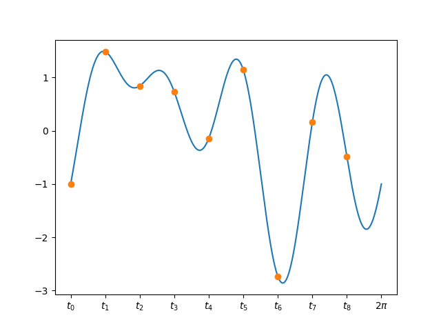
For $k = 0, \dots , 2N$. Here is an example of a function with period $T = 2\pi$ and bandwidth $N = 4$ together with the $2N+1 = 9$ samples:

Let’s try to express the value of the sample taken at the $k$-th point in terms of the Fourier series of $f(t)$. Using the Fourier expansion of $f(t)$ we have

We can simplify this expression by introducing the $2N + 1$-th root of unity $W_{2N+1}$ which is defined to be

\[ W_{2N+1} := e^{-\frac{2\pi i}{2N + 1}} \]

Our expression for $f(t_k)$ can now be expressed as

\[ f(t_k) = \sum_{n=-N}^{N} F_n W_{2N+1}^{-kn} \]

Note that this looks very similar to the expression for multiplication by a matrix whose value at $(k, n)$ is $W_{2N+1}^{-kn}$. However, the indexing from $-N$ to $N$ in the sum is a bit awkward so we will reindex using the change of variable $m = n + N$. The expression now becomes

\[ f(t_k) = \sum_{m=0}^{2N} F_{m-N} W_{2N+1}^{-k(m - N)} \]

and multiplying both sides by $W_{2N+1}^{-kN}$ gives

\begin{equation}\label{linear-eq} W_{2N+1}^{-kN}f(t_k) = \sum_{m=0}^{2N} F_{m-N} W_{2N+1}^{-km} \end{equation}

At last, the sum on the right is indeed the expression for the $k$-th row of the multiplication of a matrix and a vector which we can write out explicitly as follows

Let’s denote this matrix by $M_{2N + 1}$. It is an interesting exercise in the properties of the root of unity $W_{2N+1}$ to show that the columns of $M_{2N + 1}$ are orthogonal and that they all have a norm of $2N + 1$. From this it immediately follows that

\[ M_{2N + 1}^{-1} = \frac{1}{2N + 1} M_{2N+1}^* \]

where $M_{2N+1}^*$ denotes the conjugate transpose. By multiplying both sides of \ref{fft-matrix} with $M_{2N+1}^*$ and using the fact that the complex conjugate of $W_{2N+1}^{-1}$ is $W_{2N+1}$ we arrive at the following key equality:

The matrix appearing in the above equality is known as the discrete Fourier transform which is denoted by DFT. So we can rewrite the equality more compactly as:

\begin{equation}\label{dft} \begin{bmatrix} F_{-N} \\ F_{-N + 1} \\ F_{-N + 2} \\ \vdots \\ F_N \end{bmatrix} = \frac{1}{2N+1} \mathrm{DFT} \left( \begin{bmatrix} f(t_0) \\ W_{2N+1}^{-N}f(t_1) \\ W_{2N+1}^{-2N}f(t_2) \\ \vdots \\ W_{2N+1}^{-2N^2}f(t_{2N}) \end{bmatrix} \right) \end{equation}

The upshot of all this is that we now have an explicit expression for computing the Fourier series of the function $f(t)$ based on a list of $2N+1$ samples.

Now that we have the algorithm in hand, let’s turn to the runtime. Since the DFT is the multiplication of a matrix by a vector, the naive implementation would have complexity $\mathrm{O}(N^2)$ which is better than our original back of the envelope estimation of $\mathrm{O}(N^3)$ from the introduction, but still not fast enough for serious signal processing.

Luckily, there are some interesting symmetries in the DFT matrix which allow us to evaluate the transform with a divide and conquer approach that is appropriately called the fast Fourier transform (FFT) and which has a complexity of $\mathrm{O}(N\log(N))$. It is important to note that applying the FFT to a vector gives the same result as multiplying the vector with the DFT matrix, it is just a faster implementation of that multiplication.

The FFT is the workhorse of modern signal processing and has fast implementations in many libraries and even in hardware. We’ll work through an example using Python in the next section.

A Working Example

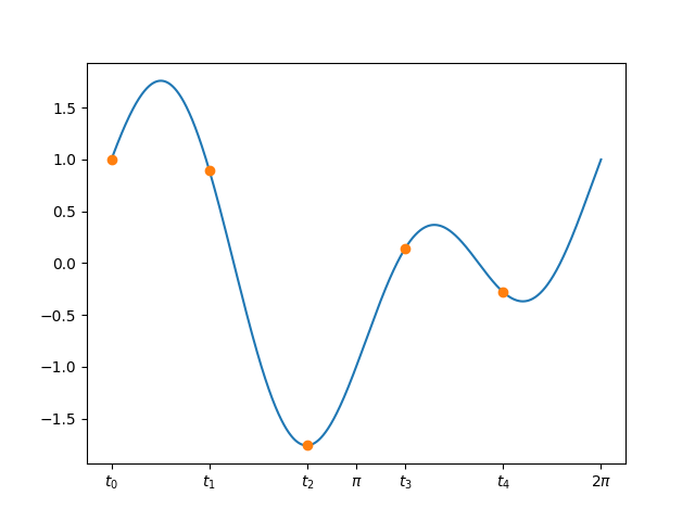
In this section we’ll put the theory of the previous sections into practice using Python. For this example we’ll consider the following function which has period $T = 2\pi$ and bandwidth $N = 2$:

\[ f(t) = \cos(t) + \sin(2t) \]

We would like to reconstruct $f$ based only on samples taken at $2N+1 = 5$ evenly spaced points $t_0, \dots, t_4$ in the interval $[0, 2\pi]$. Here is a plot of the function on the interval $[0, 2\pi]$ together with the 5 sampled points

In the following code snippet we create an array containing the samples $f(t_i)$ and then use equation \ref{dft} from the previous section to compute the Fourier series coefficients $F_n$:

import numpy as np

# Setup
# -----
N = 2  # The bandwidth of f(t)
T = 2*np.pi  # The period of f(t)

# The space between consecutive samples
T_s = T / (2*N + 1)

# The 2N+1'th root of unity
W = np.exp(-(2*np.pi*1j)/(2*N + 1))

# Generate the samples
# --------------------
# Define the function
def f(t):
    return np.cos(t) + np.sin(2*t)

# Generate the values t_0, ..., t_{2N}
t = np.array([n*T_s for n in range(2*N + 1)])

# Evaluate f(t_i) for i = 0, ..., 2N
ft = f(t)

# Reconstruct the coefficients of the Fourier
# series of f(t):  F_{-2}, F_{-1}, F_0, F_1, F_2
# using equation (3) above.
# ----------------------------------------------
scaled_ft = np.array([W**(-i*N) * ft[i]
                      for i in range(2*N + 1)])

# Apply the fast Fourier transform
F = np.fft.fft(scaled_ft) / (2*N + 1)
print("The Fourier series of f(t) is: ", F)

The output of this program is:

\[ F = [\frac{i}{2}, \frac{1}{2}, 0, \frac{1}{2}, -\frac{i}{2}] \]

Let’s verify this by plugging these coefficients into the definition of the Fourier series and check that we get $f(t)$:

Aliasing

In this final section we’ll take a look at what happens if we try to use $2N + 1$ samples to reconstruct a function whose bandwidth is greater than $N$. This is known as under-sampling since we are using fewer points than the theory allows. As we will see, a common symptom of under-sampling is that the reconstructed function has spurious low frequency components. This effect is known as aliasing.

A classic instance of aliasing is known as the wagon wheel effect. The name comes from phenomenon in which fast turning wheels in old (and even recent) movies seem to be slowly spinning backwards. To see the relationship with sampling, suppose for example that the wheel is rotating in the clockwise direction at a rate of $N$ revolutions per second. Consider the function $f(t) = \sin(-N \cdot 2\pi t)$ which describes the height of a fixed point on the wheel as a function of time. This function has a period of $1$ and a bandwidth of $N$. We can think of the process of taking a video of the wheel as measuring evenly spaced samples of $f(t)$ - one sample per frame. According to the sampling theorem, we will only be able to reconstruct the true motion of the wheel if the camera is operating at a frame rate of at least $2N+1$ frames per second. If the frame-rate is too low, the aliasing effect will introduce incorrect low frequency components which in this case manifest as a wheel which is slowly turning in the opposite direction.

We’ll now get into the technical details and understand exactly how aliasing happens. To make the equations nicer, suppose for simplicity that we are sampling a function with the following Fourier series:

\[ f(t) = \sum_{n=-N}^{N} F_n e^{n \frac{2\pi i}{T}t} + \sum_{n=N+1}^{3N+1} F_n e^{n \frac{2\pi i}{T}t} \]

In other words, in addition to the $2N+1$ non zero coefficients of a function with bandwidth $N$, there are an additional $2N+1$ non zero coefficients to the right of $N$.

Now, suppose we naively sample this function at only $2N+1$ points as if it had bandwidth $N$ and try to measure the Fourier coefficients $F_{-N}, \dots, F_N$. Similar to our derivation of the DFT above, the value of the sample $f(t_k)$ is equal to

Note the similarity of this to equation \ref{linear-eq} in our original derivation of the DFT . Similarly to there we can conclude that

This means that if we run the DFT algorithm under the assumption that the bandwidth of $f(t)$ is $N$, our estimate of the coefficient $F_n$ for $-N \leq n \leq N$ will be \(F'_n = F_n + F_{n + (2N + 1)}\). In other words, our estimates of the lower frequency components $F_{-N}, \dots, F_N$ are clouded (“aliased”) by the higher frequency components $F_{N+1}, \dots, F_{3N+1}$.

The general pattern in the case of a function $f(t)$ with arbitrarily high bandwidth is that is that our estimate of $F_n$ for $-N \leq n \leq N$ will be:

Note that even though the sum is written as infinite, in practice all but finitely many coefficients are zero since we are assuming that $f(t)$ has finite bandwidth.

In particular, even if the original signal $f(t)$ didn’t have any low frequencies at all, if we try to reconstruct if from too few samples , the reconstructed function may have low frequency components which are contributed from the higher frequencies of the original $f(t)$.

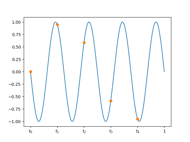
Let’s now apply this theory to a simple “wagon wheel” setup. Suppose we have a wheel that is spinning clockwise at a rate of $4$ revolutions per second. If we choose some point on the wheel, it’s height relative to the center of the wheel as a function of time is:

\[ f(t) = \sin(-4\cdot 2\pi t) \]

This function has a period of $T = 1$ and a bandwidth of $N = 4$. Its Fourier series is:

\[ f(t) = -\frac{i}{2}e^{-4\cdot 2\pi i \cdot t} + \frac{i}{2}e^{4\cdot 2\pi i \cdot t} \]

So all of it’s Fourier coefficients are zero except for $F_{-4} = -\frac{i}{2}$ and $F_{4} = \frac{i}{2}$.

By the sampling theorem, if we wanted to perfectly reconstruct this function we’d need to sample it at a rate of $2N + 1 = 9$ samples per second.

Suppose we sample this function at only $2\cdot 2 + 1 = 5$ samples per second corresponding to an incorrect bandwidth of $N’ = 2$:

According to equation \ref{aliasing-sum} and the Fourier coefficients of $f(t)$ we calculated above, if we apply the DFT algorithm to these samples we’ll recover the following (incorrect) Fourier coefficients which to avoid confusion will be denoted by $G_n$:

Plugging these coefficients into the Fourier series expression we see that the function we have measured is:

\[ g(t) = G_{-1}e^{-2\pi i \cdot t} + G_1 e^{2\pi i \cdot t} = \frac{i}{2} e^{-2\pi i \cdot t} + \frac{i}{2} e^{2\pi i \cdot t} = \sin(2\pi \cdot t) \]

This corresponds to a wheel rotating counter-clockwise (“backwards”) with a rate of just one revolution per second. Here is a plot of the original function $f(t)$ together with the samples and the reconstructed function $g(t)$:

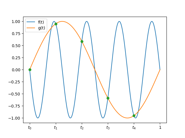
As we can see, the DFT algorithm has indeed found a function $g(t)$ with bandwidth $N’=2$ that passes through all of the $2N’+1 = 5$ samples but unfortunately this is not equal to $f(t)$ which has a higher bandwidth of $N = 4$.