Efficient Search with Markov Chains

16 Apr 2020

In this post we will discuss a method for quickly solving seemingly intractable search problems called the Metrolopis algorithm. This is one of the most popular algorithms in applied science and engineering – its use cases include optimizing the layout of circuit elements on a chip, finding a region of the genome that causes a specific disease and Google’s PageRank algorithm.

We’ll demonstrate the method via a neat application to encryption which is due to Persi Diaconis. We will then try to understand why the method works and see that it can be explained using the beautiful theory of Markov chains.

Substitution Ciphers

A substitution cipher is a simple type of encryption in which each letter in the message is replaced with a different letter using a lookup table.

Here is an example of a cipher:

a b c d e f g h i j k l m n o p q r s t u v w x y z . , ? ! _
l f _ o r , y h q s v e c ? g a t . w j n z p d ! m x u b k i

When we apply this cipher to a message, each letter in the top row will be replaced by the letter below it. For instance, every a in the message will be replaced by an l. As an example, this is what we get when we apply the cipher to line from Alice and Wonderland:

plaintext:  the rabbit hole went straight on like a tunnel for some way
ciphertext: jhri.lffqjihgeripr?jiwj.lqyhjig?ieqvrilijn??rei,g.iwgcripl!

We are following the convention of calling the original message the plaintext and the encrypted message the ciphertext. In order to decode the ciphertext, we must find the key which tells us how to convert letters in the ciphertext back to the original letters in the plaintext. For example, since the cipher turns each q into an t, the key would convert t back to q. In our example the full key would be:

a b c d e f g h i j k l m n o p q r s t u v w x y z . , ? ! _
p ? m x l b o h _ t ! a z u d w i e j q , k s . g v r f n y c

You can check that if we apply this key to the ciphertext we indeed recover the original plaintext. For example, the first three letters of the ciphertext are jhr. According to the key, we should replace j with t, h with h and r with e. Together this gives us the word the which is indeed the first word of the plaintext.

It will be convenient in what follows to adopt the following notation. We will denote a key by a function \[ K: \{\mathrm{characters}\} \rightarrow \{\mathrm{characters}\} \]

Given a string $S=c_1c_2\dots c_N$, applying a key $K$ to the string gives us a new string \[ K(S) := K(c_1)K(c_2)\dots K(c_N) \]

Using the key in our example above: $K(\mathrm{jhr}) = \mathrm{the}$.

It is well known that finding the key is not very difficult, which means that the substitution cipher is not a particularly strong form of encryption. These days it is only useful as a way of making text slightly harder to read such as when you want to avoid giving out unsolicited spoilers. The reason for this is that in the English language, certain letters are more common that others. For instance, it is likely that the most frequent characters in the ciphertext should be converted to e, t, a or o.

However, our goal today is not to get into the details of substitution ciphers or the statistics of the English language but rather to introduce the Metropolis algorithm which we will use to quickly find the key.

In general, the input to the Metropolis algorithm is a set of states $x_1,\dots,x_N$ and a function $L$ that assigns each state a likelihood $L(x_i)$. The output of the algorithm is the state (or states) with the highest likelihood.

Of course, if the number of states is reasonably small and $L$ is easy to evaluate then we can simply calculate $L(x_i)$ for each $i$ and find the maximum. But in many cases of interest the number of states is a large number like $N=10^{50}$ and $L$ is a nontrivial function. Amazingly, in these situations the Metropolis algorithm frequently manages to find the optimal $x_i$ despite calculating the likelihoods of only a handful of states.

In the following few sections we will use this algorithm to decode a message by searching for the key which, when applied to the ciphertext, produces the sequence of characters which is most likely to be English. In this setup, the set of states consists of all possible keys. Since each permutation of the alphabet (together with some punctuation) is a valid key, there are around $30! \sim 10^{32}$ states. We will calculate the likelihood of a key by applying it to the ciphertext and measuring how similar the result is to English with the help of a simple language model.

In the next section we will build a basic language model and show how it can be used to estimate the likelihood that a given piece of text is in English.

After that we will introduce the Metropolis algorithm and use it, together with our language model, to write a short program that breaks substitution ciphers in less than a second.

A Simple Language Model

In this section we will develop a model that measures the resemblance of a sequence of characters to English. Our model will be based on the probabilities of consecutive characters.

We begin by considering the function $\mathrm{PairProb}(c_1, c_2)$ which is defined to be equal to the probability of seeing the character $c_2$ assuming that the previous character was $c_1$. For example $\mathrm{PairProb}(\mathrm{q}, \mathrm{u})$ should be relatively high compared to $\mathrm{PairProb}(\mathrm{q}, \mathrm{x})$ because when we see the letter q, it is very likely that the next letter is a u. We will shortly address the question of how to estimate $\mathrm{PairProb}$.

Once we have a way of calculating $\mathrm{PairProb}(c_1, c_2)$ for each pair of letters $c_1$ and $c_2$, we can estimate the likelihood of a sequence of characters $c_1c_2\dots c_N$ by multiplying the probabilities of each consecutive pair: \[ \mathrm{Likelihood}(c_1\dots c_N) := \prod_{i=1}^{N-1}\mathrm{PairProb}(c_i,c_{i+1}) \]

In practice, to avoid overflow issues we will typically be interested in the loglikelihood: \[ \mathrm{LogLikelihood}(c_1\dots c_N) := \log(\mathrm{Likelihood}(c_1\dots c_N)) = \sum_{i=1}^{N-1}\log (\mathrm{PairProb}(c_i,c_{i+1})) \]

Let’s write some code that estimates $\mathrm{PairProb}(c_1,c_2)$ using a large text file and use it to compute the loglikelihood of an arbitrary sequence of characters.

To begin, we must be explicit about which characters we will include in our calculations. We will be using lowercase letters, common punctuation and of course the useful “space”:

CHARACTERS = "abcdefghijklmnopqrstuvwxyz.,?! "

It will also be useful to refer to characters based on their index in CHARACTERS. Here are some handy utility functions to that end.

import collections
import numpy as np

def build_char_to_idx_dict():
    """Build a dictionary that maps characters to their index in our list
       CHARACTERS. Characters that are not in the list will be mapped to
       len(CHARACTERS)-1 which represents a space.
    """
    char_to_idx = collections.defaultdict(lambda: len(CHARACTERS) - 1)
    char_to_idx.update({char: i for i, char in enumerate(CHARACTERS)})    
    return char_to_idx

def text_to_idx(text, char_to_idx):
    """Convert each character in the text to an index using char_to_idx."""
    return np.array([char_to_idx[char] for char in text.lower()], np.int32)

def idx_to_text(text_idx):
    """Convert each index to a character using the CHARACTERS array."""
    return ''.join([CHARACTERS[idx] for idx in text_idx])

We will now write a method that computes the table $\log \mathrm{PairProb}(c_1, c_2)$ using a text file.

def update_pair_counts(line, pair_counts, char_to_idx):
    """Use the line to update the counts of consecutive pairs."""
    for first, second in zip(line, line[1:]):
        pair_counts[char_to_idx[first], char_to_idx[second]] += 1

def compute_pair_log_probabilities(text_filename):
    """Use the text in the file to compute the array P defined by:
       P[i, j] := log probability of CHARACTERS[j] following CHARACTERS[i]
    """
    char_to_idx = build_char_to_idx_dict()
    P = np.zeros((len(CHARACTERS), len(CHARACTERS)))
    
    with open(text_filename, 'r') as fh:
        for line in fh:
            update_pair_counts(line.lower(), P, char_to_idx)
    
    # Normalize the rows to sum to 1
    P = P / np.sum(P, axis=1).reshape((-1, 1))
    
    # Replace the zeros with the smallest non zero value
    min_prob = P[P > 0].min()
    P[P == 0] = min_prob
    
    return np.log(P)

Finally, we can use the table returned by compute_pair_log_probabilities to compute the loglikelihood of a string.

def compute_log_likelihood(text_idx, pair_log_probs):
    """Compute the loglikelihood of a list of character indices
       using the specified array of pairwise log probabilities.
    """
    first = text_idx[:-1]
    second = text_idx[1:]
    return np.sum(pair_log_probs[first, second])

We’ll now demonstrate these methods by generating a table of pairwise log probabilities from War and Peace which you can download here

>>> pair_log_probs = compute_pair_log_probabilities("war_and_peace.txt")
>>> char_to_idx = build_char_to_idx_dict()
>>> print(pair_log_probs[char_to_idx['q'], char_to_idx['u']])
-0.0008583691514160856
>>> print(pair_log_probs[char_to_idx['q'], char_to_idx['x']])
-12.330111627440097

As expected, after seeing a q, it is very likely that the next character is a u.

Let’s play around with the compute_log_likelihood method. Here is the loglikelihood of the first sentence of Harry Potter:

>>> text = """Mr. and Mrs. Dursley, of number four, Privet Drive, were proud to say that
they were perfectly normal, thank you very much."""
>>> text_idx = text_to_idx(text, char_to_idx)
>>> print(compute_log_likelihood(text_idx, pair_log_probs))
-306.70425959388507

In comparison, here is the loglikelihood of a random sequence of characters with the same length:

text = """hc!zvohq?oh.yemahxrevfux?e?c lqx!obgqfkmxfmzz.lrx?nsscrgjjumuxdk,rasiddfh.
ibjlofdeegztenosxsjqqy?g!l. buunrcjzitpiqrizg.wta"""
>>> text_idx = text_to_idx(text, char_to_idx)
>>> print(compute_log_likelihood(text_idx, pair_log_probs))
-928.5920308990139

So at the very least, our model gives Harry Potter a high likelihood of being English compared to random gibberish.

The Metropolis Algorithm

We will now return to our original goal of reading messages that were encrypted with a substitution cipher. As we discussed earlier, in order to read a ciphertext message we must find the key which tells us how to convert characters in the ciphertext back to their original values.

Intuitively, we can assess the quality of a key by applying it to the ciphertext and evaluating the result with our language model. For instance, the true key converts the ciphertext back to the original plaintext which should have a high likelihood if our language model is doing its job. Conversely, applying a random key would result in a garbled string of characters which, as we saw earlier, should have a relatively low likelihood.

With this in mind, our strategy for reading a ciphertext $C=c_1c_2\dots c_N$ will be to find the key $K$ that maximizes the loglikelihood of $K(C)$ which by definition is equal to \[ \mathrm{LogLikelihood}(K(C)) = \sum_{i=1}^{N-1}\log (\mathrm{PairProb}(K(c_i),K(c_{i+1}))) \]

If we had infinite computing power, we could simply enumerate all possible keys and find the one with the highest likelihood. Unfortunately, there are approximately $10^{32}$ keys which renders brute force impractical.

Instead, we will use the following “hill climbing” strategy which we will later identify as a special case of the Metrolopis algorithm.

1. Choose a random key $K$.
2. Swap two random outputs of $K$ to get a new key $K’$.
3. Let $r = \frac{\mathrm{Likelihood}(K’(C))}{\mathrm{Likelihood}(K(C))}$. If $r \geq 1$, meaning that $K’$ has a higher likelihood than $K’$, update $K := K’$.
4. If $r < 1$, flip a weighted coin where heads has weight $r$. If it comes up heads, update $K := K’$.
5. If we have not exceeded 5000 iterations, go back to step 2. Otherwise, return $K$.

Generally speaking, we start at a random key and keep trying to improve it by making random changes to its outputs. If the new key is better we take it. And even if it’s worse, there is a small probability that we still take it. This last part is important since it prevents us from being trapped at a local minimum.

Amazingly, this simple algorithm almost always manages to find the correct key after just 5000 iterations!

Here is some code that implements the algorithm:

def apply_key(key, text_idx):
    return substitution[text_idx]


def random_transposition(N):
    """Generate a random pair of integers (i, j)
       such that i!=j and 0 <= i,j < N.
    """
    return np.random.choice(N, size=(2,), replace=False)


def apply_transposition(sigma, permutation):
    """Apply the transposition sigma=(i,j) to the permutation."""
    output = permutation.copy()
    output[sigma[0]], output[sigma[1]] = output[sigma[1]], output[sigma[0]]
    return output


def find_key(ciphertext_idx, pair_log_probs, n_iter=5000):
    """Find the key that decodes the ciphertext using the language
       model defined by pair_log_probs.
    """
    key = np.random.permutation(len(CHARACTERS))
    text_idx = apply_key(key, ciphertext_idx)
    key_ll = compute_log_likelihood(text_idx, pair_log_probs)
    
    best_key = key
    best_key_ll = key_ll
    
    for i in range(n_iter):
        sigma = random_transposition(len(key))
        new_key = apply_transposition(sigma, key)
        text_idx = apply_key(new_key, ciphertext_idx)
        new_key_ll = compute_log_likelihood(text_idx, pair_log_probs)

        r = np.exp(new_key_ll - key_ll)
        if np.random.uniform() < r:
            key = new_key
            key_ll = new_key_ll
            
            if key_ll > best_key_ll:
                best_key = key
                best_key_ll = key_ll
            
    return best_key

Let’s use the algorithm to decrypt a message:

>>> ciphertext = """
otqway..jowt,gqwdqhowuoayj!tow,hwgjzqwywo?hhqgwi,awu,xqwdyskwyhvwotqhwvjmmqvwu?v
vqhgswv,dhkwu,wu?vvqhgswotyowygjpqwtyvwh,owywx,xqhowo,wotjhzwy.,?owuo,mmjh!wtqau
qgiw.qi,aqwutqwi,?hvwtqauqgiwiyggjh!wv,dhwywcqaswvqqmwdqgglwwqjotqawotqwdqggwdyu
wcqaswvqqmkw,awutqwiqggwcqaswug,dgskwi,awutqwtyvwmgqhosw,iwojxqwyuwutqwdqhowv,dh
wo,wg,,zwy.,?owtqawyhvwo,wd,hvqawdtyowdyuw!,jh!wo,wtymmqhwhqeolwijauokwutqwoajqv
wo,wg,,zwv,dhwyhvwxyzqw,?owdtyowutqwdyuwp,xjh!wo,kw.?owjowdyuwo,,wvyazwo,wuqqwyh
sotjh!wwotqhwutqwg,,zqvwyowotqwujvquw,iwotqwdqggkwyhvwh,ojpqvwotyowotqswdqaqwijg
gqvwdjotwp?m.,yavuwyhvw.,,zwutqgcquwwtqaqwyhvwotqaqwutqwuydwxymuwyhvwmjpo?aquwt?
h!w?m,hwmq!ulwutqwo,,zwv,dhwywryawia,xw,hqw,iwotqwutqgcquwyuwutqwmyuuqvwwjowdyuw
gy.qggqvw,ayh!qwxyaxygyvqkw.?owo,wtqaw!aqyowvjuymm,jhoxqhowjowdyuwqxmoswwutqwvjv
wh,owgjzqwo,wva,mwotqwryawi,awiqyaw,iwzjggjh!wu,xq.,vsw?hvqahqyotkwu,wxyhy!qvwo,
wm?owjowjho,w,hqw,iwotqwp?m.,yavuwyuwutqwiqggwmyuowjolwwdqggbwot,?!towygjpqwo,wt
qauqgikwyioqawu?ptwywiyggwyuwotjukwjwutyggwotjhzwh,otjh!w,iwo?x.gjh!wv,dhwuoyjau
bwt,dw.aycqwotqswggwyggwotjhzwxqwyowt,xqbwdtskwjwd,?gvhwowuyswyhsotjh!wy.,?owjok
wqcqhwjiwjwiqggw,iiwotqwo,mw,iwotqwt,?uqbwwdtjptwdyuwcqaswgjzqgswoa?qlww
"""

>>> char_to_idx = build_char_to_idx_dict()
>>> pair_log_probs = compute_pair_log_probabilities("war_and_peace.txt")
>>> ciphertext_idx = encode(ciphertext, char_to_idx)
>>> key = find_key(ciphertext_idx, pair_log_probs, n_iter=5000)
>>> plaintext_idx = apply_key(key, ciphertext_idx)
>>> plaintext = idx_to_text(plaintext_idx)
>>> print(plaintext)
the rabbit hole went straight on like a tunnel for some way, and then dipped sud
denly down, so suddenly that alice had not a moment to think about stopping hers
elf before she found herself falling down a very deep well.  either the well was
 very deep, or she fell very slowly, for she had plenty of time as she went down
 to look about her and to wonder what was going to happen next. first, she tried
 to look down and make out what she was coming to, but it was too dark to see an
ything  then she looked at the sides of the well, and noticed that they were fil
led with cupboards and book shelves  here and there she saw maps and pictures hu
ng upon pegs. she took down a jar from one of the shelves as she passed  it was 
labelled orange marmalade, but to her great disappointment it was empty  she did
 not like to drop the jar for fear of killing somebody underneath, so managed to
 put it into one of the cupboards as she fell past it.  well! thought alice to h
erself, after such a fall as this, i shall think nothing of tumbling down stairs
! how brave they ll all think me at home! why, i wouldn t say anything about it,
 even if i fell off the top of the house!  which was very likely true.

Clearly the algorithm found the correct key, and we have recovered the original message which was a passage from Alice and Wonderland. Furthermore, the call to find_key completes in less than a second which is not surprising given that we have only 5000 iterations.

Here is a plot of the loglikelihood of the key at each iteration:

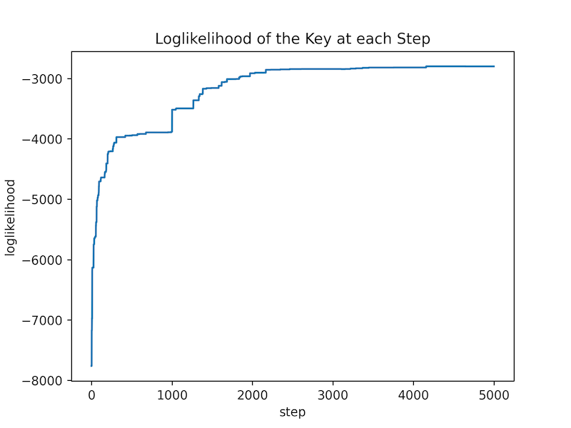
As you can see, the algorithm converges quite quickly.

If you look at the implementation of find_key you’ll see that the only parts that are specific to the context of substitution ciphers are:

1. The random_transposition and apply_transposition methods which allow us to jump to a random neighbor of the current key.
2. The compute_log_likelihood method which evaluates the quality of a key.

This suggests that the algorithm can work more generally in a setting in which we have many states $x_1,\dots,x_n$ and a measure of the value of each state, together with a way of sampling nearby states. In this type of setting, we can apply an analog of find_key to find the state with the highest value.

Indeed, this is called the Metropolis Algorithm which has many applications in applied science and engineering.

In the next few sections we will explain why the algorithm works. We’ll start by introducing the theory of Markov chains which was developed specifically to understand what happens if you randomly jump between a set of states. In the last section we’ll apply this theory to the Metropolis algorithm.

Markov Chains

What is a Markov Chain

A Markov chain describes a process which is defined by a set of states $\{x_1,\dots,x_n\}$ and an array of transition probabilities $[p_{ij}]_{1 \leq i,j \leq n}$. The process starts at some initial state $x_\mathrm{initial}$. If we are currently at state $x_i$, the probability that we will move to state $x_j$ is $p_{ij}$.

Here is an example from Wikipedia involving the following simplified weather model:

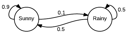
In this model there are only two states - $S$ and $R$ representing sunny and rainy weather respectively. The transition matrix is: \[ P = \begin{bmatrix} 0.9 & 0.1 \\ 0.5 & 0.5 \end{bmatrix} \]

The first row of $P$ tells us the transition probabilities assuming that the weather is currently sunny. In that case, the next day will be sunny with probability $p_{11} = 0.9$ and rainy with probability $p_{12} = 0.1$. Similarly, the bottom row tells us that if it is rainy today, then tomorrow it is equally likely to be sunny or rainy.

We call this process a chain because we can use it to simulate a random sequence (or “chain”) of states. Here is some code that samples a sequence from a Markov chain with two states like the one in our example.

def sample_chain(P, initial_state, n_steps):
    """Sample n_steps iterations of a Markov chain with two states."""
    chain = [initial_state]
    for _ in range(n_steps-1):
        state = chain[-1]

        # Go to state 0 with probability P[state, 0]
        if np.random.random() < P[state, 0]:
            chain.append(0)
        else:
            chain.append(1)
    
    return chain

We use it to generate 5 simulations of 50 days of weather using our model:

>>> P = np.array([[0.9, 0.1], [0.5, 0.5]])
>>> state_names = ['S', 'R']

>>> for _ in range(5):
>>>    chain = sample_chain(P, initial_state=0, n_steps=50)
>>>    print(''.join([state_names[s] for s in chain]))
SSSRSSSSSSSSSSSSSSSSSSSSSSSSSSSSSSSSSSSSSSSSSSSSSS
SSSSSSSSSSSSSSSSSSSSRRRSSSSRRRRSSSSSSSSRSSRRRRSSSS
SSSSSSSSSSSSSSSRRRRRSSSSRSSSSSSSSSSRRRRRSSRRSSSSSS
SSRRRRRSSSSSSSSSSSSSSSSSSSSSSRRSSSSSSSSSSSSSSSRSSS
SSSRRRRSSSSSRSSSSSSSSSSSSRSSSSSSSSSSSRRRSSSSRRRRRR

The Stationary Distribution

When presented with a Markov chain, we are typically interested questions about the long term behavior such as: What is the probability that in 50 days the weather will be sunny? Based on the 5 samples above we may expect the answer to be around $\frac{4}{5} = 0.8$, but how can we calculate the precise answer?

For starters, let’s figure out the probability $p^{(2)}_{11}$ of it being sunny in two days from now assuming it is sunny today. There are two ways for this to happen. One option is for it to be sunny tomorrow and also sunny the day after. According to the transition matrix (or the diagram) this will happen with a $p_{11}p_{11} = 0.9\cdot 0.9 = 0.81$ probability. The other option is for it to be rainy tomorrow and then sunny the day after. This latter possibility occurs with a $p_{12}p_{21} = 0.1\cdot 0.5=0.05$ probability. Putting both options together we find the the probability of it being sunny in two days from now is: \[ p^{(2)}_{11} = p_{11}p_{11} + p_{12}p_{21} = 0.81 + 0.05 = 0.86 \]

You may recognize this as the expression for $(P^2)_{11}$ - the top left element in the matrix $P^2$. In general, if the current state is $x_i$, then the probability that we will be in state $j$ after two steps is $(P^2)_{ij}$. In our example: \[ P^2 = \begin{bmatrix} 0.86 & 0.14 \\ 0.7 & 0.3 \end{bmatrix} \]

From the bottom row we can see that if it is rainy today, the probability of it being rainy in two days from now is $0.3$.

In fact, this rule holds for any number of transitions. Specifically, if the current state is $x_i$ then the probability that we will reach state $x_j$ after $n$ transitions is $(P^n)_{ij}$.

Let’s see what this implies for our weather forecasts: \[ P^3 = \begin{bmatrix} 0.833 & 0.167 \\ 0.833 & 0.167 \end{bmatrix} \]

Interestingly, both rows of $P^3$ are equal (to 3 decimal points). This means that the probability of being sunny or rainy in three days does not depend on the todays weather! For example, the probability of it being sunny in three days is $0.833$, regardless of whether it is sunny or rainy today.

Further calculations show that for all $n \geq 3$,

\[ P^n = \begin{bmatrix} 0.833 & 0.167 \\ 0.833 & 0.167 \end{bmatrix} \]

So after three days the probability of it being sunny converges to $0.833$, and this holds for any number of days greater than $3$.

To test this out, let’s generate 10000 sequences of 20 days of weather and check which fraction of them are sunny:

>>> N = 10000
>>> num_sunny = 0
>>> for _ in range(N):
>>>    state = np.random.randint(0,2)
>>>    chain = sample_chain(P, initial_state=state, n_steps=20)
>>>    if chain[-1] == 0:
>>>       num_sunny += 1
>>>    
>>> print(f"Fraction of chains that ended sunny: {num_sunny / N}")
0.8305

We get the answer of $0.8305$ which is pretty close to our theoretical calculation of $0.833$.

The probability distribution $\begin{bmatrix}0.833 & 0.167\end{bmatrix}$ is called the stationary distribution because after a sufficiently large number of steps we reach this distribution and from then on it stops changing.

Regular Markov Chains

It is natural to wonder if all Markov chains have a stationary distribution. In order to see that this is false, consider the following alternative transition matrix for our weather model: \[ P’ = \begin{bmatrix} 0 & 1 \\ 1 & 0 \end{bmatrix} \]

This transition matrix implies that sunny days are always followed by rainy days and vice versa. Therefore, if today is sunny, our state in $n$ days from now will be sunny if $n$ is even and rainy if $n$ is odd. This means that the Markov chain has no stationary distribution because the probability of being in any given state jumps around over time rather than converging to a fixed value.

Fortunately, a common type of Markov chains called regular Markov chains do have stationary distributions.

Definition: A Markov chain with transition matrix $P$ is called regular if there exists an integer $n$ such that all of the entries of $P^n$ are greater than zero.

In other words, a Markov chain is regular if there exists an integer $n$ such that it is possible to get from every state to every other state in $n$ steps.

Our original weather forecasting Markov chain is clearly regular since the positivity condition holds for $P$ itself.

We can now state a key theorem in theory of Markov chains which formalizes the fact that every regular Markov chain has a stationary distribution:

For example, we already saw that our weather forecasting Markov chain was regular so the theorem applies. Indeed, we’ve already seen that:

\[ \lim_{n\rightarrow\infty}P^n = \begin{bmatrix} 0.833 & 0.167 \\ 0.833 & 0.167 \end{bmatrix} \]

so in this case, $W = \begin{bmatrix} 0.833 & 0.167 \\ 0.833 & 0.167 \end{bmatrix}$ and $\mathbf{w} = \begin{bmatrix}0.833 & 0.167\end{bmatrix}$. As we mentioned earlier, the row matrix $\mathbf{w}$ is called the stationary distribution.

Proving this theorem is outside the scope of this post, but if you are curious I suggest looking at chapter 11 of the excellent book Introduction to Probability by Grinstead and Snell.

Calculating the Stationary Distribution

As we have seen, every regular Markov chain has a stationary distribution. This is great because once we know this distribution, we can predict the probability of landing in any state after a large number of iterations without actually having to simulate the chain. For instance, in our weather example we know that the probability of it being sunny in $1000$ days is $0.833$, regardless of what the weather is today.

But how can we calculate the stationary distribution? The naive way is to calculate $\lim_{n\rightarrow\infty}P^n$ by taking higher and higher powers of $P$. But if $P$ is large, this will not be computationally tractable.

It turns out that there is a faster way to do this which takes advantage of the following important theorem.

We will prove this theorem at the end of the section. For now, let’s apply this theorem to our weather example. In that case: \[ \mathbf{w}P = \begin{bmatrix}0.833 & 0.167 \end{bmatrix} \begin{bmatrix} 0.9 & 0.1 \\ 0.5 & 0.5 \end{bmatrix} = \begin{bmatrix}0.833 & 0.167\end{bmatrix} = \mathbf{w}
\]

as implied by the theorem.

There are two common ways by which this theorem helps us calculate the stationary distribution $\mathbf{w}$.

The first way uses the fact that according to the theorem, $\mathbf{w}$ is the unique left eigenvector (up to a scalar) of $P$ with an eigenvalue of $1$. Therefore, we can find $\mathbf{w}$ using an off-the-shelf linear algebra library to compute the eigenvectors of $P$.

However, in many cases of practical interest $P$ is so large that even calculating eigenvectors is not feasible. In those cases, is is sometimes possible to guess that the stationary distribution is some vector $\mathbf{x}$. According to the theorem, we can verify our guess by checking if $\mathbf{x}P = \mathbf{x}$. This may sound a bit silly, but this is the method we will use in our analysis of the Metropolis algorithm in the following section.

Proof of Theorem 2

We will now prove theorem 2. Feel free to skip ahead if you are more interested in seeing how the theorem is used to analyze the Metropolis algorithm.

First let’s show that if $\mathbf{w}$ is the stationary distribution then $\mathbf{w}P=\mathbf{w}$. By theorem 1 we know that \[ \lim_{n\rightarrow\infty}P^n = W \]

where all the rows of $W$ are equal to the stationary distribution $\mathbf{w}$. Now note that

In summary we’ve shown that $WP = W$. But since each row of $W$ is equal to $\mathbf{w}$, it follows that $\mathbf{w}P = \mathbf{w}$.

For the other direction, suppose that $\mathbf{x}P = \mathbf{x}$ for some row vector $\mathbf{x}$. It easily follows by induction that $\mathbf{x}P^n = \mathbf{x}$ for all $n$. Therefore, \[ \mathbf{x}W = \mathbf{x}\lim_{n\rightarrow\infty}P^n = \lim_{n\rightarrow\infty}\mathbf{x}P^n = \lim_{n\rightarrow\infty}\mathbf{x} = \mathbf{x} \] which means that $\mathbf{x}W = \mathbf{x}$.

Let $r$ be equal to the sum of the components of $\mathbf{x}$. Since all of the rows of $W$ are equal to $\mathbf{w}$, it is easy to see that $\mathbf{x}W = r\mathbf{w}$.

Together, with our previous observation that $\mathbf{x}W = \mathbf{x}$ it follows that $\mathbf{x} = r\mathbf{w}$. Indeed, $\mathbf{x}$ is proportional to $\mathbf{w}$ which is what we wanted to show.

Why the Metropolis Algorithm Works

We are finally in a position to understand the logic behind the Metropolis algorithm. Recall that the algorithm works by starting at an initial key, and then at each stage we with some probability either stay at the same key or move to a random neighboring key. We can now recognize this rule as describing a Markov chain $M$ whose states are the possible keys $K_1,\dots,K_n$. We will soon describe this chain in more detail.

The fundamental idea behind the Metropolis algorithm is that $M$ is a regular Markov chain, and that its stationary distribution is proportional to a row vector whose $i$-th element is equal to the likelihood of the key $K_i$. By the definition of the stationary distribution, this means that once we run enough iterations of the chain, or in this case, the Metropolis algorithm, the probability of landing on a key will be proportional to its likelihood. In particular, we have a good chance of landing on the key with the highest likelihood!

The remainder of this section will be devoted to describing the Markov chain $M$, and proving the properties we alluded to above.

The Transition Matrix $P$

In this section we will compute the transition matrix $P$ for the Markov chain $M$.

First let’s nail down some notation. Let $C=c_1\dots c_m$ denote our ciphertext. Recall that we earlier defined the likelihood of a key $K$ to be the likelihood that the language model assigns to $K(C)$: \[ \mathrm{Likelihood}(K(C)) = \prod_{i=1}^{N-1}\mathrm{PairProb}(K(c_i),K(c_{i+1})) \]

To facilitate notation, we will use the abbreviation \[ L(K) := \mathrm{Likelihood}(K(C)) \]

In addition, let $A$ denote the number of characters in the alphabet.

Finally, we will define $\mathrm{Nbd}(K)$, short for the neighborhood of $K$, to be the set of keys that can be obtained by applying a transposition to $K$. Note that for all $i$, the size of the neighborhood is \[ |\mathrm{Nbd}(K)| = \binom{A}{2} \]

This is because there is exactly one transposition for each pair of distinct characters in the alphabet.

Let us now calculate the coefficients of the transition matrix $P_{ij}$ of the Markov chain $M$. By definition, $P_{ij}$ is equal to the probability of moving from the key $K_i$ to the key $K_j$. We will determine these probabilities by following the update rule of the Metropolis algorithm. There are 4 cases to cover.

Since we only jump to keys in the neighborhood of $K_i$, if $K_j \notin \mathrm{Nbd}(K_i)$ then $P_{ij} = 0$.

Now let’s focus the cases where $K_j \in \mathrm{Nbd}(K_i)$. Since there are $\binom{A}{2}$ elements in the neighborhood, the chance that the algorithm considers $K_j$ is $\binom{A}{2}^{-1}$. Once we’ve selected $K_j$ there are two possibilities.

• If $L(K_j) \geq L(K_i)$ then we always go to $K_j$. So in this case $P_{ij} = \binom{A}{2}^{-1}$.
• If $L(K_j) < L(K_i)$ then we go to $K_j$ with probability $L(K_j) / L(K_i)$. So in this case, $P_{ij} = \frac{L(K_j)}{L(K_i)}\binom{A}{2}^{-1}$.

Let last remaining option is when $i=j$. But since we know that $\sum_jP_{ij} = 1$, the value of $P_{ii}$ is determined by the probabilities we have already calculated: $P_{ii} = 1 - \sum_{j\neq i}P_{ij}$.

This concludes the description of the transition matrix $P$.

The Stationary Distribution

In this section we will show that the Markov chain is regular and identify its stationary distribution.

For the regularity, note that it is possible to turn any key $K$ into any other key $K’$ with at most $A$ transpositions. We simply have to swap each of the $A$ outputs of $K$ with the corresponding output of $K’$. If you would like to understand this part in more detail, I’d suggest checking out the Wikipedia article on transpositions. The upshot of this is that it is possible to get between any two states in $A$ steps, which by definition implies that the Markov chain is regular.

Since our Markov chain $M$ is regular, by theorem 1 it must have a stationary distribution. We boldly make the following assertion.

As we mentioned earlier, this claim is the fundamental reason that the Metropolis algorithm works. To reiterate, if the stationary distribution of $M$ is $\mathbf{w}$ then, by definition, if we start from a random key and apply many iterations of the Markov chain, then the probability of ending up at key $K_i$ is proportional to $\mathbf{w}_i$. According to the claim, $\mathbf{w}_i=L(K_i)$. Therefore, the probability of ending up at $K_i$ is proportional to its likelihood $L(K_i)$.

But we defined the Markov chain so that making a step in the chain is exactly the same as doing an iteration of the Metropolis algorithm. Therefore, at the end of the algorithm the probability of ending up at $K_i$ is also proportional $L(K_i)$. In particular, there is a high chance that we end up at the the true key which has by far the greatest likelihood.

Proof of Claim 1

In this section we will prove claim 1.

According to theorem 2 it suffices to show that \begin{equation}\label{eq:eigen-vec} \mathbf{w}P = \mathbf{w} \end{equation}

Given the complexity of $P$ this doesn’t seem a lot easier. However, it actually follows quite easily from the following lemma:

Before proving this lemma let’s use it to prove equation \ref{eq:eigen-vec} and thus claim 1. Indeed, note that it follows from the lemma that that for any $i$:

Let’s unpack this. Equality $(1)$ is just the definition of matrix multiplication. Equality $(2)$ follows from the definition of $\mathbf{w}$. The key nontrivial step is $(3)$ which uses lemma 1. Finally, $(4)$ holds because the sum of any row of a transition matrix is equal to $1$.

In summary, we have shown that for all $i$, $(\mathbf{w}P)_i = \mathbf{w}_i$. Therefore $\mathbf{w}P = \mathbf{w}$ which is what we wanted to show.

Now all that remains is to prove lemma 1. We will break it down into the same four cases that we encountered while calculating $P_{ij}$.

We’ll start with the easy cases. For starters, if $K_j$ is not a neighbor of $K_i$ then $P_{ij}=P_{ji}=0$ and the lemma is trivial. The lemma is also obvious when $i=j$.

Now consider what happens if $K_j$ is in the neighborhood of $K_i$. If $L(K_i) \geq L(K_j)$ then by our earlier calculations we know that $P_{ij}=\frac{L(K_j)}{L(K_i)}\binom{A}{2}^{-1}$ and $P_{ji}=\binom{A}{2}^{-1}$. Therefore \[ L(K_i)P_{ij} = L(K_i)\frac{L(K_j)}{L(K_i)}\binom{A}{2}^{-1} = L(K_j)\binom{A}{2}^{-1} = L(K_j)P_{ji} \]

The case where $L(K_i) < L(K_j)$ is similar. This concludes the proof of the lemma.